The first step of the solution is to use the Biot number to see if the pin can be modeled as a single lump or if the problem must be broken down into many smaller elements.
Equation 8.20, B_{i} =\frac{h_{c}L }{k} defines the Biot number, where L is the characteristic length for the problem, k is the thermal conductivity of aluminum, and h_{c} is the convective heat transfer coefficient for this problem.
The characteristic length is that dimension along which one is likely to see variations in temperature. In this case, the length (0.01 m), rather than the diameter, is the proper dimension to use. Thermal properties of aluminum are easily found in handbooks and are summarized in Table 8.1.
| Property |
Value |
Units |
| Density |
2707 |
{Kg}/{m^{3} } |
| Thermal conductivity |
220 |
{W}/{m^{ \ \omicron }C } |
| Specific heat \left(c_{p} \right) |
896 |
{J}/{Kg^{ \ \omicron }C } |
As discussed in Subsection 8.2.2, the determination of convective heat transfer coefficients can be a very difficult task; however, for simple geometries, heat transfer textbooks provide reasonable ranges for these coefficients. For this geometry, it was decided that a value of 20{W}/{m^{2 \ \omicron }C } was a reasonable estimate.
Therefore the Biot number is
B_{i} =\frac{h_{c} L}{k}=\frac{\left(20\right) \left(0.01\right) }{220} =0.001,
which would indicate that a lumped model for the entire pin is adequate. The essential assumption to move forward from this point is that the entire pin is at a uniform temperature throughout the analysis. If part of the information you hoped to extract from this analysis is the temperature distribution along the pin, then the problem will still have to be broken down to smaller elements.
Beginning with a simple single-lump model, we note the following energy balance:
\left ( \begin{matrix} rate\ of\ heat\ stored \\ in\ the\ pin \end{matrix} \right ) =\left ( \begin{matrix} rate\ of\ heat \\ conducted\ through\ base \end{matrix} \right )-\left ( \begin{matrix} rate\ of\ heat \\ convected\ to\ air \end{matrix} \right ), (8.27)
from which the single differential equation can be written:
C_{h} \frac{dT_{pin} }{dt} =\frac{1}{R_{hk} } \left(T_{base}-T_{pin} \right) -\frac{1}{R_{hc} }\left(T_{pin}-T_{a} \right), (8.28)
where
C_{h} =\rho c_{p} V=\left(2707\right) \left(896\right) \left(3.14\times 10^{-8} \right) =0.0762 J/ ^{\omicron }C
R_{hk} =\frac{L}{kA_{k} } =\frac{0.005}{\left(220\right)\left(3.14\times 10^{-6} \right) } =7.23^{\omicron } {C}/{W},
R_{hc} =\frac{1}{h_{c} A_{c} } =\frac{1}{\left(20\right)\left(6.28\times 10^{-5} \right) } =796^{\omicron } {C}/{W}.
Note that the length used in the conductive term represents the length from the base of the pin to its center whereas the area A_{k} is the circular (cross-section) area of the base of the pin through which the conduction takes place. On the other hand, the area used to compute the convective resistance, A_{c}, is the surface area of the pin exposed to the air.
Substituting the numerical values and putting the equation in standard form leads to the following equation:
\frac{dT_{pin} }{dt} +1.83T_{pin} =1.81T_{base}+0.017T_{a}. (8.29)
Following the techniques discussed in Chap. 4, one can find the solution of this differential equation:
T_{pin} \left(t\right) =100-75e^{-1.83t} (8.30)
Figure 8.4 shows the response of the temperature of the pin for 3 s following a sudden change in the base temperature.
Although the low value of the Biot number indicates that the time response computed with a single lumped model is relatively accurate and that the entire pin will be approximately at the same temperature, some temperature variation along the length of the pin will no doubt exist. If this variation is of interest (and it often is for heat transfer analysis), a more detailed approach is called for.
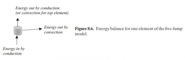
When the pin is divided into five equal segments along its length, the result is a stack of cylinders, as seen in Fig. 8.5.
Figure 8.6 shows a sketch of one of the pin elements, indicating the paths through which thermal energy is transmitted. As shown in the one-lump model, an energy balance for each element results in a first-order differential equation. Because there are five elements, this model is represented by five first-order equations. These equations are subsequently shown in state-space form.
\frac{d}{dt} T_{1} =\frac{1}{C_{h} } \left[-\left(\frac{1}{R_{hk0} }+\frac{1}{R_{hk} } +\frac{1}{R_{hc} } \right) T_{1}+\frac{1}{R_{hk} }T_{2}+ \frac{1}{R_{hk0} }T_{base}+\frac{1}{R_{hc} }T_{a} \right] , (8.31)
\frac{d}{dt} T_{2}=\frac{1}{C_{h} }\left[\frac{1}{R_{hk} }T_{1}-\left(\frac{2}{R_{hk} }+\frac{1}{R_{hc} }\right)T_{2}+\frac{1}{R_{hk} }T_{3} +\frac{1}{R_{hc} }T_{a} \right] , (8.32)
\frac{d}{dt} T_{3}=\frac{1}{C_{h} }\left[\frac{1}{R_{hk} }T_{2}-\left(\frac{2}{R_{hk} }+\frac{1}{R_{hc} }\right)T_{3}+\frac{1}{R_{hk} }T_{4} +\frac{1}{R_{hc} }T_{a} \right] (8.33)
\frac{d}{dt} T_{4}=\frac{1}{C_{h} }\left[\frac{1}{R_{hk} }T_{3}-\left(\frac{2}{R_{hk} }+\frac{1}{R_{hc} }\right)T_{4}+\frac{1}{R_{hk} }T_{5} +\frac{1}{R_{hc} }T_{a} \right] (8.34)
\frac{d}{dt} T_{5}=\frac{1}{C_{h} }\left[\frac{1}{R_{hk} }T_{4}-\left(\frac{1}{R_{hk} }+\frac{1}{R_{hc} }+\frac{1}{R_{hce} }\right)T_{5} +\left(\frac{1}{R_{hc} }+\frac{1}{R_{hce} }\right) T_{a}\right] , (8.35)
where the thermal capacitance of an element C_{H}, conductive resistances R_{hk}, and convective resistances R_{hc}, are given by the following expressions:
C_{h} =\rho c_{p} V=\left(2707\right) \left(896\right) \left(6.28\times 10^{-9} \right) =0.0152\frac{J}{^{\omicron }C } ,thermal capacitance of an
element;
R_{hko} =\frac{L_{0} }{kA_{k} } =\frac{0.001}{\left(220\right)\left(3.14\times 10^{-6} \right) } =1.45\frac{^{\omicron }C }{W} ,conductive resistance between element 1 and base;
R_{hk} =\frac{L }{kA_{k} } =\frac{0.002}{\left(220\right)\left(3.14\times 10^{-6} \right) } =2.89\frac{^{\omicron }C }{W} ,conductive resistance between
adjacent elements;
R_{hc} =\frac{L }{h_{c} A_{c} } =\frac{1}{\left(20\right)\left(1.26\times 10^{-5} \right) } =3968\frac{^{\omicron }C }{W} ,convective resistance between
element sides and the environment;
R_{hce} =\frac{L }{h_{c} A_{ce} } =\frac{1}{\left(20\right)\left(3.14\times 10^{-6} \right) } =16,000\frac{^{\omicron }C }{W} ,convective resistance between the top surface of element 5 and
the environment.
Although conventional analytical methods can be used to solve these equations, computer methods are much more convenient. Figure 8.7 shows the Simulink model that solves a state-space linear model with two inputs. The parameters of the model are embedded in the state matrices. Because the main state matrix is a 5 × 5 matrix, it is best to write an m-file to set up the system matrices, thus allowing the user to more easily make modifications and experiment with the model. The m-file corresponding to this model is shown in Table 8.2.
The temperature response that is in the center of the five lines represents the temperature of the center element \left(T_{3} \right). This response can be compared directly with the single-lump response computed in Fig. 8.4. It is interesting to note that the responses are similar, but by no means identical, showing that the single-lump model does not completely represent the complexity of the pin.
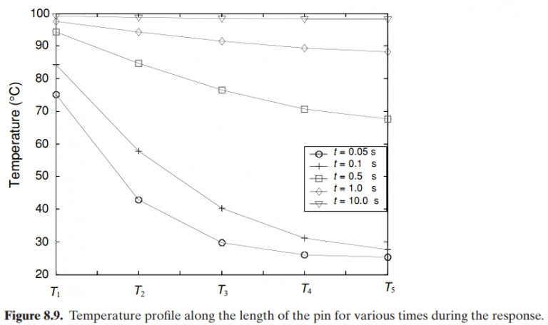
Finally, Figure 8.9 represents the variation of temperature along the pin for various points in the time response. It is important to note that, even though the Biot number for the single-lump model indicated that the temperature could be assumed
to be uniform along the pin, that conclusion would not be valid for the transient portion of the response (less than 1 s).