Find the end displacement δ in each of the members illustrated in Fig. 4.6.

Question

Find the end displacement in each of the members illustrated in Fig. 4.6.

Accepted Answer

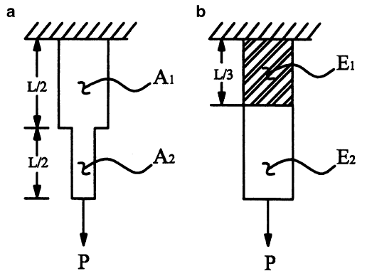
The first structure (Fig. 4.6a) is homogenous and subject to a constant axial load P, but it does not have a constant cross-sectional area. The area changes abruptly from [latex]A_{1}[/latex] to [latex]A_{2}[/latex] at [latex]x=L/2.[/latex] Thus, [latex]A=A(x)[/latex] and the end displace-ment is determined via

[latex] u_{x}(x)-u_{x}(0)=\int_{0}^{x}{\frac{P}{A(x)E}dx }\rightarrow \delta =u_{x}(0)+\frac{P}{E}\int_{0}^{L}{\frac{dx}{A(x)} }.[/latex]

The integral must be separated at the point of discontinuity in the cross-sectional area to give the following results [with [latex]u_{x}(0)=0[/latex] via a boundary condition]:

[latex] \delta =\frac{P}{E}\int_{0}^{L/2}{\frac{dx}{A_{1}}+\frac{P}{E} }\int_{L/2}^{L}{\frac{dx}{A_{2}}\rightarrow \delta }=\frac{P}{A_{1}E}\int_{0}^{L/2}{dx+\frac{P}{A_{2}E} }\int_{L/2}^{L}{dx},[/latex]

or

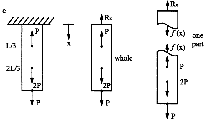
[latex] \delta =\frac{PL}{2A_{1}E}+\frac{PL}{2A_{2}E}=\frac{PL}{2E}\left(\frac{1}{A_{1}}+\frac{1}{A_{2}} \right).[/latex]

The second structure (Fig. 4.6b) has a constant cross-sectional area and is subjected to a constant axial load P, but it is not homogenous. The material FIGURE 4.6 Axially loaded rods having a nonconstant cross section (panel a), a nonconstant material composition (panel b), and multiple applied loads (panel c). Although we need to draw free-body diagrams of the whole and multiple parts for each case, we show only the free- ody diagram of the whole structure and one free-body diagram for a part of the rod of panel c.

properties change at x=L/3 from the wall. Therefore, E=E(x) and the displacement becomes

[latex] u_{x}(x)-u_{x}(0)=\frac{P}{A}\int_{0}^{x}{\frac{dx}{E(x)} }\rightarrow \delta =u_{x}(0)+\frac{P}{A}\int_{0}^{L}{\frac{dx}{E(x)} }.[/latex]

Again dividing the integration over judicious domains, we have

[latex] \delta =\frac{P}{A}\int_{0}^{L/3}{\frac{dx}{E_{1}} }+\frac{P}{A}\int_{L/3}^{L}{\frac{dx}{E_{2}} },[/latex]

where [latex]u_{x}(x=0)=0[/latex] again. Hence, we find

[latex] \delta =\frac{PL}{3AE_{1}}+\frac{2PL}{3AE_{2}}=\frac{PL}{3A}\left(\frac{1}{E_{1}}+\frac{2}{E_{2}} \right).[/latex]

For the third problem (Fig. 4.6c), we must first solve the statics problem.Equilibrium of the whole requires that the reaction force [latex]R_{x}[/latex] be given by

[latex] -R_{x}-P+2P+P=0\rightarrow R_{x}=2P,[/latex]

whereas equilibrium of parts requires that we consider three separate cuts. For the first part,

[latex] -R_{x}+f(x)=0\rightarrow f(x)=2P, 0\leq x\lt \frac{L}{3}.[/latex]

Similarly, for the second part,

[latex] -R_{x}-P+f(x)=0\rightarrow f(x)=3P, \frac{L}{3}\lt x\lt \frac{2L}{3}.[/latex]

Finally, for the third required part,

[latex] -R_{x}-P+2P+f(x)=0\rightarrow f(x)=P, \frac{2L}{3}\lt x\leq L.[/latex]

Indeed, the last result can be seen easily given a small part near the end. Regardless, given constants E and A and [latex]u_{x}(x=0),[/latex] we have

[latex] \delta =\frac{1}{AE}\left(\int_{0}^{L/3}{2P dx}+\int_{L/3}^{2L/3}{3P dx}+\int_{2L/3}^{L}{P dx} \right)=2\frac{PL}{AE}.[/latex]

Question 4.2: Find the end displacement δ in each of the members illustrat...

Related Answered Questions