(a) The effective potential is (Equation 4.53):
-\frac{\hbar^{2}}{2 m_{e}} \frac{d^{2} u}{d r^{2}}+\left[-\frac{e^{2}}{4 \pi \epsilon_{0}} \frac{1}{r}+\frac{\hbar^{2}}{2 m_{e}} \frac{\ell(\ell+1)}{r^{2}}\right] u=E u (4.53).
V(r)=-\frac{e^{2}}{4 \pi \epsilon_{0}} \frac{1}{r}+\frac{\hbar^{2}}{2 m_{e}} \frac{\ell(\ell+1)}{r^{2}} .
Now V_{j}=V\left(r_{j}\right), r_{j}=j \Delta r, \Delta r=\frac{b}{N+1}, \lambda=\frac{\hbar^{2}}{2 m_{e}(\Delta r)^{2}} , so
v_{j} \equiv \frac{V_{j}}{\lambda}=\frac{2 m_{e}}{\hbar^{2}} \frac{b^{2}}{(N+1)^{2}}\left[-\frac{e^{2}}{4 \pi \epsilon_{0}} \frac{(N+1)}{j b}+\frac{\hbar^{2}}{2 m_{e}} \frac{\ell(\ell+1)(N+1)^{2}}{j^{2} b^{2}}\right] .
=-\frac{2 m_{e} e^{2}}{4 \pi \epsilon_{0} \hbar^{2}} \frac{b}{(N+1)} \frac{1}{j}+\frac{\ell(\ell+1)}{j^{2}}=-\frac{2 b}{a(N+1)} \frac{1}{j}+\frac{\ell(\ell+1)}{j^{2}}=-\frac{2 \beta}{j}+\frac{\ell(\ell+1)}{j^{2}} .
(b) \Delta r \ll a \ll b \Rightarrow \frac{b}{N+1} \ll \frac{b}{(N+1) \beta} \ll b \Rightarrow 1 \ll(1 / \beta) \ll N+1 \sim N , Note that u(0) = 0 (Equation 4.59), and u(b) = 0, so we have the same boundary conditions as Problem 2.61.
u(\rho) \sim C \rho^{\ell+1} (4.59).
\underline{\ell=0}
h =\text { Table }[\operatorname{If}[i==j, \quad 2-(1 /(25 j)), 0],\{i, 1000\},\{j, 1000\}] .
k =\text { Table }[\operatorname{If}[i==j+1,-1,0],\{i, 1000\},\{j, 1000\}] .
m =\text { Table }[\operatorname{If}[i== j -1,-1,0],\{ i , 1000\},\{ j , 1000\}] .
p=\text { Table }[h[[i, j]]+k[[i, j]]+m[[i, j]],\{i, 1000\},\{j, 1000\}] .
EIG = Eigenvalues[N[p]].
EVE = Eigenvectors[N[p]].
ListLinePlot [EVE[[994]], PlotRange – >\{0,0.11\} ].
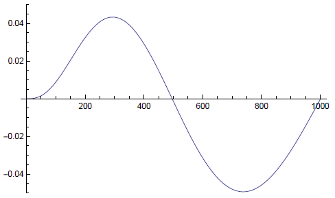
ListLinePlot [EVE[[997]], PlotRange – >\{-0.05,0.07\} ].
ListLinePlot [EVE[[999]], PlotRange – >\{-0.05,0.07\} ].
EIG[[994]]
-0.00039996
EIG[[997]]
-0.0000999873
EIG[[999]]
-0.0000399639.
To get the actual energy (see Equation 2.199), multiply by \lambda=\frac{\hbar^{2}(N+1)^{2}}{2 m_{e} b^{2}}=\frac{\hbar^{2}}{2 m_{e} a^{2}} \frac{1}{\beta^{2}}=-E_{1} / \beta^{2} , in other words, we must multiply by 1 / \beta^{2}=2500 , and the result will be the energy in units of 13.6 eV (the exact answer, of course, would be -1/n² = -1,-0.25,-0.1111):
H \equiv \lambda\left(\begin{array}{cccccc} & & & & & & \\ & -1 & \left(2+v_{j-1}\right) & -1 & 0 & 0 & \\ & 0 & -1 & \left(2+v_{j}\right) & -1 & 0 & \\ & 0 & 0 & -1 & \left(2+v_{j+1}\right) & -1 & \\ & & & & & & \ddots \end{array}\right) (2.199).
-0.00039996 \times(2500)=0.9999 E_{1},-0.000099987 \times(2500)=0.24997 E_{1},-0.000039964 \times(2500)=0.09991 E_{1} .
The first two are pretty good; the third is a bit off (but notice from the graph that the wave function has not dropped to zero well before r = b).
\underline{\ell=1 } .
h =\text { Table }\left[\operatorname{If}\left[i==j, 2-(1 /(25 j))+\left(2 /\left(j^{\wedge} 2\right)\right), 0\right],\{ i , 1000\},\{j, 1000\}\right] .
k =\text { Table }[\operatorname{If}[i= =j +1,-1,0],\{i, 1000\},\{ j , 1000\}] .
p=\text { Table }[h[[[i, j]]+k[[i, j]]+m[[i, j]],\{i, 1000\},\{j, 1000\}] .
EIG = Eigenvalues[N[p]].
EVE = Eigenvectors[N[p]].
ListLinePlot [EVE[[999]], PlotRange – >\{0,0.065\} ].
ListLinePlot [EVE[[999]], PlotRange – >\{-0.04,0.06\} ].
ListLinePlot [EVE[[1000]], PlotRange – >\{-0.06,0.05\} ].
EIG[[997]] * 2500
-0.249991
EIG[[999]] * 2500
-0.103278
EIG[[1000]] * 2500
0.0158618
For {\ell=1 } the lowest state is n = 2, so the exact energies (in units of E_1 ) are 0.25, 0.1111, and 0.0625.
0.24999E_1, 0.10328E_1, -0.015862E_1.
The first is good; the second is a bit off (but notice from the graph that the wave function has not dropped to zero well before r = b), and the third is terrible (wrong sign).
\underline{\ell=2}
h=\text { Table }[\text { If }[i==j, 2-(1 /(25 j))+(6 /(j \wedge 2)), 0],\{i, 1000\},\{j, 1000\}] .
k =\operatorname{Table}[\operatorname{If}[ i == j +1,-1,0],\{ i , 1000\},\{ j , 1000\}] .
m =\text { Table }[\operatorname{If}[ i == j -1,-1,0],\{ i , 1000\},\{ j , 1000\}] .
p =\operatorname{Table}[h[[i, j]]+k[[i, j]]+m[[i, j]],\{i, 1000\},\{j, 1000\}] .
EIG = Eigenvalues[N[p]].
EVE = Eigenvectors[N[p]].
ListLinePlot [EVE[[999]], PlotRange – >\{0,0.065\} ].
ListLinePlot [EVE[[1000]], PlotRange – >\{-0.05,0.05\} ].
ListLinePlot [EVE[[998]], PlotRange – >\{-0.06,0.05\} ].
EIG[[999]] * 2500
-0.107958
EIG[[1000]] * 2500
-0.0112765
EIG[[998]] * 2500
0.135962
\text { For } \ell=2 \text { the lowest state is } n=3 \text {, so the exact energies (in units of } E_{1} \text { ) are 0.1111, 0.0625, and } 0.04 \text {. }
0.10796E_1, 0.011277E_1, -0.13596E_1 .
The first is OK; the second is a way off, and the third is terrible (wrong sign). But in all three cases the wave function has not dropped to zero well before r = b. To improve the results we would a substantially larger b.