One way to obtain the allowed energies of a potential well numerically is to turn the Schrödinger equation into a matrix equation, by discretizing the variable x. Slice the relevant interval at evenly spaced points (xj) , with xj + 1 - xj ≡ Δ x , and let ψj ≡ ψ(xj) (likewise Vj ≡ V(xj)) . Then d ψ/

Question

One way to obtain the allowed energies of a potential well numerically is to turn the Schrödinger equation into a matrix equation, by discretizing the variable x. Slice the relevant interval at evenly spaced points [latex] \left\{x_{j} ight\} [/latex] , with [latex] x_{j+1}-x_{j} \equiv \Delta x [/latex] , and let [latex] ψ_j ≡ ψ(x_j)[/latex] (likewise [latex] V_j ≡ V(x_j)[/latex]) . Then

[latex] \frac{d \psi}{d x} \approx \frac{\psi_{j+1}-\psi_{j}}{\Delta x}, \frac{d^{2} \psi}{d x^{2}} \approx \frac{\left(\psi_{j+1}-\psi_{j} ight)-\left(\psi_{j}-\psi_{j-1} ight)}{(\Delta x)^{2}}=\frac{\psi_{j+1}-2 \psi_{j}+\psi_{j-1}}{(\Delta x)^{2}} [/latex] (2.195).

(The approximation presumably improves as Δx decreases.) The discretized Schrödinger equation reads

[latex] -\frac{\hbar^{2}}{2 m}\left(\frac{\psi_{j+1}-2 \psi_{j}+\psi_{j-1}}{(\Delta x)^{2}} ight)+V_{j} \psi_{j}=E \psi_{j} [/latex]. (2.196)

or

[latex] -\lambda \psi_{j+1}+\left(2 \lambda+V_{j} ight) \psi_{j}-\lambda \psi_{j-1}=E \psi_{j}, \quad ext { where } \quad \lambda \equiv \frac{\hbar^{2}}{2 m(\Delta x)^{2}} [/latex]. (2.197).

In matrix form,

[latex] H \Psi=E \Psi [/latex] (2.198).

where (letting [latex] v_{j} \equiv V_{j} / \lambda [/latex]).

[latex] H \equiv \lambda\left(\begin{array}{cccccc} \ddots & & & & & & \ & -1 & \left(2+v_{j-1} ight) & -1 & 0 & 0 & \ & 0 & -1 & \left(2+v_{j} ight) & -1 & 0 & \ & 0 & 0 & -1 & \left(2+v_{j+1} ight) & -1 & \ & & & & & & \ddots \end{array} ight) [/latex] (2.199).

and

[latex] \Psi \equiv\left(\begin{array}{c} \vdots \ \psi_{j-1} \ \psi_{j} \ \psi_{j+1} \ \vdots \end{array} ight) [/latex] (2.200) .

(what goes in the upper left and lower right corners of H depends on the boundary conditions, as we shall see). Evidently the allowed energies are the eigenvalues of the matrix H (or would be, in the limit Δx → 0 ).

Apply this method to the infinite square well. Chop the interval (0 ≤ x ≤a) into N+1 equal segments (so that Δx = a / (N+1)), letting [latex] x_0 ≡ 0 [/latex] and [latex] x_{N+1} \equiv a [/latex]. The boundary conditions fix [latex] \psi_{0}=\psi_{N+1}=0 [/latex], leaving

[latex] \Psi \equiv\left(\begin{array}{c} \psi_{1} \ \vdots \ \psi_{N} \end{array} ight) [/latex] (2.201).

(a) Construct the N × N matrix H ,for N=1 ,N=2, and N=3. (Make sure you are correctly representing Equation 2.197 for the special cases [latex] j=1 ext { and } j=N [/latex].)

(b) Find the eigenvalues of H for these three cases “by hand,” and compare them with the exact allowed energies (Equation 2.30).

[latex] E_{n}=\frac{\hbar^{2} k_{n}^{2}}{2 m}=\frac{n^{2} \pi^{2} \hbar^{2}}{2 m a^{2}} [/latex] (2.30).

(c) Using a computer (Mathematica’s Eigenvalues package will do it) find the five lowest eigenvalues numerically for N=10 and N=100, and compare the exact energies.

(d) Plot (by hand) the eigenvectors for N=1 , 2 and 3, nd (by computer, Eigenvectors) the first three eigenvectors for N=10 and N=100.

Accepted Answer

(a) From Equation 2.197:

[latex] -\lambda \psi_{j+1}+\left(2 \lambda+V_{j} ight) \psi_{j}-\lambda \psi_{j-1}=E \psi_{j}, \quad ext { where } \quad \lambda \equiv \frac{\hbar^{2}}{2 m(\Delta x)^{2}} [/latex]. (2.197).

[latex] N=1: j=1:-\lambda \cancel{\psi_{2}}+(2 \lambda) \psi_{1}-\lambda \cancel{\psi_{0}}=E \psi_{1} \quad \Rightarrow \quad H =(2 \lambda) [/latex].

[latex] N=2:\left\{\begin{array}{l} j=1:-\lambda \psi_{2}+(2 \lambda) \psi_{1}-\lambda \cancel{\psi_{0}}=E \psi_{1} \ j=2:-\lambda \cancel{\psi_{3}}+(2 \lambda) \psi_{2}-\lambda \psi_{1}=E \psi_{2} \end{array} \quad \Rightarrow ight. H =\left(\begin{array}{cc} 2 \lambda & -\lambda \ -\lambda & 2 \lambda \end{array} ight) [/latex].

[latex] N=3:\left\{\begin{array}{l} j=1:-\lambda \psi_{2}+(2 \lambda) \psi_{1}-\lambda \cancel{\psi_{0}}=E \psi_{1} \ j=2:-\lambda \psi_{3}+(2 \lambda) \psi_{2}-\lambda \psi_{1}=E \psi_{2} \ j=3:-\lambda \cancel{\psi_{4}}+(2 \lambda) \psi_{3}-\lambda \psi_{2}=E \psi_{2} \end{array} \Rightarrow ight. H =\left(\begin{array}{ccc} 2 \lambda & -\lambda & 0 \ -\lambda & 2 \lambda & -\lambda \ 0 & -\lambda & 2 \lambda \end{array} ight) [/latex].

(b) Denote the eigenvalues by [latex] ilde{E}_{n} [/latex]:

[latex] N=1: ilde{E}_{1}=2 \lambda=\frac{2 \hbar^{2}}{2 m(a / 2)^{2}}=\frac{8 \hbar^{2}}{2 m a^{2}} [/latex]. The exact energies are [latex] E_{n}=\frac{n^{2} \pi^{2} \hbar^{2}}{2 m a^{2}}, ext { so } E_{1}=\frac{\pi^{2} \hbar^{2}}{2 m a^{2}} [/latex]; the agreement is not too bad: [latex] 8 \approx \pi^{2}=9.87 [/latex].

N = 2 :

[latex] \operatorname{det}\left(\begin{array}{cc} 2 \lambda- ilde{E} & -\lambda \ -\lambda & 2 \lambda- ilde{E} \end{array} ight)=0 \Rightarrow(2 \lambda- ilde{E})^{2}-\lambda^{2}=0 \Rightarrow 2 \lambda- ilde{E}=\pm \lambda [/latex].

[latex] ilde{E}_{1}=2 \lambda-\lambda=\lambda=\frac{\hbar^{2}}{2 m(a / 3)^{2}}=\frac{9 \hbar^{2}}{2 m a^{2}} [/latex] . This is better: 9 is closer to π² than 8 was.

[latex] ilde{E}_{2}=2 \lambda+\lambda=3 \lambda=\frac{3 \hbar^{2}}{2 m(a / 3)^{2}}=\frac{27 \hbar^{2}}{2 m a^{2}} [/latex]. The exact answer has 4π² = 39.5 instead of 27.

N = 3 :

[latex] \operatorname{det}\left(\begin{array}{ccc} 2 \lambda- ilde{E} & -\lambda & 0 \ -\lambda & 2 \lambda- ilde{E} & -\lambda \ 0 & -\lambda & 2 \lambda- ilde{E}
\end{array} ight)=0 \Rightarrow(2 \lambda- ilde{E})^{3}-2 \lambda^{2}(2 \lambda- ilde{E})=0 \Rightarrow 2 \lambda- ilde{E}=0 ext { or } 2 \lambda- ilde{E}=\pm \sqrt{2} \lambda [/latex].

[latex] ilde{E}_{1}=2 \lambda-\sqrt{2} \lambda=\lambda(2-\sqrt{2})=\frac{(2-\sqrt{2}) \hbar^{2}}{2 m(a / 4)^{2}}=\frac{16(2-\sqrt{2}) \hbar^{2}}{2 m a^{2}} [/latex]. This is better yet: [latex] 16(2-\sqrt{2})=9.37 [/latex].

[latex] ilde{E}_{2}=2 \lambda=\frac{2 \hbar^{2}}{2 m(a / 4)^{2}}=\frac{32 \hbar^{2}}{2 m a^{2}} [/latex] . Improving: the exact answer is 4π² = 39.5 instead of 32.

[latex] ilde{E}_{3}=2 \lambda+\sqrt{2} \lambda=\lambda(2+\sqrt{2})=\frac{(2+\sqrt{2}) \hbar^{2}}{2 m(a / 4)^{2}}=\frac{16(2+\sqrt{2}) \hbar^{2}}{2 m a^{2}} ; 16(2+\sqrt{2})=54.6 \approx 9 \pi^{2}=88.8 [/latex].

(c)

h = Table [If [i == j, 2 λ, 0], [latex] \{i, 10\},\{j, 10\} [/latex]].

k = Table [If [i == j+1, - λ, 0], [latex] \{i, 10\},\{j, 10\} [/latex]].

m = Table [If [i == j-1, - λ, 0], [latex] \{i, 10\},\{j, 10\} [/latex]].

p = Table [h [ [i , j]] + k [[i,j]] + m [[i,j]] , [latex] \{i, 10\},\{j, 10\} [/latex]].

P = MatrixForm[%]

[latex] \left(\begin{array}{cccccccccc} 2 \lambda & -\lambda & 0 & 0 & 0 & 0 & 0 & 0 & 0 & 0 \ -\lambda & 2 \lambda & -\lambda & 0 & 0 & 0 & 0 & 0 & 0 & 0 \ 0 & -\lambda & 2 \lambda & -\lambda & 0 & 0 & 0 & 0 & 0 & 0 \ 0 & 0 & -\lambda & 2 \lambda & -\lambda & 0 & 0 & 0 & 0 & 0 \ 0 & 0 & 0 & -\lambda & 2 \lambda & -\lambda & 0 & 0 & 0 & 0 \ 0 & 0 & 0 & 0 & -\lambda & 2 \lambda & -\lambda & 0 & 0 & 0 \ 0 & 0 & 0 & 0 & 0 & -\lambda & 2 \lambda & -\lambda & 0 & 0 \ 0 & 0 & 0 & 0 & 0 & 0 & -\lambda & 2 \lambda & -\lambda & 0 \ 0 & 0 & 0 & 0 & 0 & 0 & 0 & -\lambda & 2 \lambda & -\lambda \ 0 & 0 & 0 & 0 & 0 & 0 & 0 & 0 & -\lambda & 2 \lambda \end{array} ight) [/latex].

λ=1

1

EIG = Eigenvalues [N[p]].

[latex] \left\{83.91899, 3.68251, 3.30972, 2.83083, 2.28463,1.71537, 1.16917, 0.690279, 0.317493, 0.0810141 ight\} [/latex].

To get the eigenvalues, multiply by [latex] \lambda=\frac{\hbar^{2}}{2 m(a / 11)^{2}}=\left(\frac{121}{\pi^{2}} ight) E_{1} [/latex]:

121 * EIG / (π^2).

[latex] \left\{848.0462, 45.147, 40.5767, 34.7056, 28.0092, 21.0302, 14.3339, 8.46272, 3.89242, 0.993221 ight\} [/latex].

Thus the lowest five eigenvalues, in units of [latex] E_1 [/latex], are 0.9932, 3.8924, 8.4627, 14.3339, 21.0302, as compared to the exact values 1, 4, 9, 16, 25. Doing the same for N = 100:

h = Table [If [i == j, 2 λ, 0], [latex] \{i, 100\},\{j, 100\} [/latex]].

k = Table [If [i == j+1, - λ, 0], [latex] \{i, 100\},\{j, 100\} [/latex]].

m = Table [If [i == j-1, - λ, 0], [latex] \{i, 100\},\{j, 100\} [/latex]].

p = Table [h [ [i , j]] + k [[i,j]] + m [[i,j]] , [latex] \{i, 100\},\{j, 100\} [/latex]].

λ=1

1

EIG = Eigenvalues[N[p]]

10201 * EIG/(π^2).

{ 4133.31 , 4130.31 , 4125.32 , 4118.33 , 4109.36 , 4098.41 , 4085.5 , 4070.64 , 4053.84 , 4035.11 ,

4014.49 , 3991.97 , 3967.6 , 3941.39 , 3913.36 , 3883.55 , 3851.98 , 3818.69 , 3783.7,3747.04,

3708.77,3668.9,3627.49,3584.57,3540.18,3494.36, 3447.16,3398.63,3348.81,3297.75,

3245.5,3192.11,3137.63,3082.12,3025.62,2968.2,2909.9,2850.79,2790.92,2730.35,

2669.14,2607.35,2545.03,2482.25,2419.07,2355.55,2291.76,2227.74,2163.57,2099.3,

2035.011970.74,1906.57,1842.55,1778.75,1715.24,1652.06,1589.28,1526.96,1465.17,1403.96,

1343.39,1283.52,1224.41,1166.11,1108.69,1052.19, 996.679,942.201,888.81,836.559,

785.499,735.679,687.147,639.95,594.133,549.742,506.819,465.405,425.541,387.265,

350.614,315.624,282.328,250.76,220.948,192.922,166.71,142.336,119.824,99.1963,

80.4724,63.6704,48.8067,35.8956,24.9496,15.9794,8.99347,3.99871,0.999919 }.

This time the lowest five eigenvalues are 0.9999, 3.9987, 8.9934, 15.9794, 24.9496.

(d) Always, [latex] \psi_{0}=\psi_{N+1}=0 [/latex] ;might as well set λ=1 for the last part.

N = 1 : [latex] 2 \psi_{1}= ilde{E} \psi_{1}, ilde{E}_{1}=2 [/latex] Up to normalization:

[latex] N=2:\left(\begin{array}{cc} 2 & -1 \ -1 & 2 \end{array} ight)\left(\begin{array}{l} \psi_{1} \ \psi_{2} \end{array} ight)= ilde{E}\left(\begin{array}{l} \psi_{1} \ \psi_{2} \end{array} ight) \Rightarrow 2 \psi_{1}-\psi_{2}= ilde{E} \psi_{1} ext { and }-\psi_{1}+2 \psi_{2}= ilde{E} \psi_{2} [/latex].

[latex] n=1: ilde{E}_{1}=1 \Rightarrow 2 \psi_{1}-\psi_{2}=\psi_{1} \Rightarrow \psi_{2}=\psi_{1} [/latex].

[latex] n=2: ilde{E}_{2}=3 \Rightarrow 2 \psi_{1}-\psi_{2}=3 \psi_{1} \Rightarrow \psi_{2}=-\psi_{1} [/latex].

[latex] N=3:\left(\begin{array}{ccc} 2 & -1 & 0 \ -1 & 2 & -1 \ 0 & -1 & 2 \end{array} ight)\left(\begin{array}{l} \psi_{1} \ \psi_{2} \ \psi_{3} \end{array} ight)= ilde{E}\left(\begin{array}{l} \psi_{1} \ \psi_{2} \ \psi_{3} \end{array} ight) \Rightarrow 2 \psi_{1}-\psi_{2}= ilde{E} \psi_{1},-\psi_{1}+2 \psi_{2}-\psi_{3}= ilde{E} \psi_{2},-\psi_{2}+2 \psi_{3}= ilde{E} \psi_{3} [/latex].

[latex] n=1: ilde{E}_{1}=2-\sqrt{2} \Rightarrow 2 \psi_{1}-\psi_{2}=(2-\sqrt{2}) \psi_{1} \Rightarrow \psi_{2}=\sqrt{2} \psi_{1} [/latex];

[latex] -\psi_{1}+2 \psi_{2}-\psi_{3}=(2-\sqrt{2}) \psi_{2} \Rightarrow \psi_{1}+\psi_{3}=\sqrt{2} \psi_{2}=2 \psi_{1} \Rightarrow \psi_{3}=\psi_{1} [/latex].

[latex] n=2: ilde{E}_{2}=2 \Rightarrow 2 \psi_{1}-\psi_{2}=2 \psi_{1} \Rightarrow \psi_{2}=0 ;-\psi_{1}+2 \psi_{2}-\psi_{3}=2 \psi_{2} \Rightarrow \psi_{3}=-\psi_{1} [/latex].

[latex] n=3: ilde{E}_{3}=2+\sqrt{2} \Rightarrow 2 \psi_{1}-\psi_{2}=(2+\sqrt{2}) \psi_{1} \Rightarrow \psi_{2}=-\sqrt{2} \psi_{1} [/latex];

[latex] -\psi_{1}+2 \psi_{2}-\psi_{3}=(2+\sqrt{2}) \psi_{2} \Rightarrow \psi_{1}+\psi_{3}=-\sqrt{2} \psi_{2}=2 \psi_{1} \Rightarrow \psi_{3}=\psi_{1} [/latex].

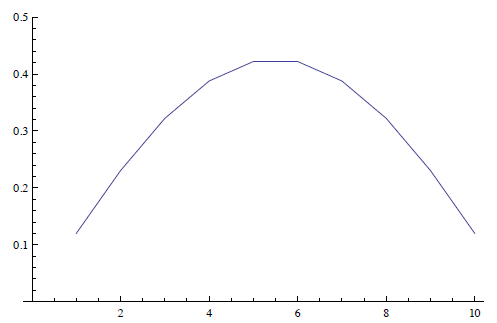
For N = 10 we get

EVE = Eigenvectors [N[p]]

ListLinePlot [EVE[[10]], PlotRange → [latex] \left\{0,0.5 ight\}[/latex] ].

ListLinePlot [EVE[[9]], PlotRange → [latex] \left\{-0.5,0.5 ight\}[/latex] ].

ListLinePlot [EVE[[8]], PlotRange → [latex] \left\{-0.5,0.5 ight\}[/latex] ].

and for N = 100

EVE = Eigenvectors [N[p]]

ListLinePlot [EVE[[100]], PlotRange → [latex] \left\{0,0.2 ight\}[/latex] ].

ListLinePlot [EVE[[99]], PlotRange → [latex] \left\{-0.2,0.2 ight\}[/latex] ].

ListLinePlot [EVE[[98]], PlotRange → [latex] \left\{-0.2,0.2 ight\}[/latex] ].

Question 2.61: One way to obtain the allowed energies of a potential well n...

Related Answered Questions