Question 12.2: Prepare Bode diagram curves for the first-order system descr...

Step 1. Transforming to the s domain yields

sY(s)+\frac{Y(s)}{\tau } =\frac{kX(s)}{\tau }  .      (12.29)

The system transfer function is

T(s)+\frac{Y(s)}{X(s) } =\frac{k}{\tau s+1 }  .     (12.30)

Step 2. The sinusoidal transfer function is

T(j\omega )=T(s ){\mid _{s=j\omega } }  =\frac{k}{j\omega \tau +1 }  .      (12.31)

Step 3. To simplify the process of obtaining expressions for T(ω) and \phi_{T} (ω), note that T(jω) can be presented as a ratio of complex functions N(jω) and D(jω):

T(j\omega )= \frac{N_{(j\omega )} }{D_{(j\omega )} } =\frac{N(\omega )e^{j\phi N(\omega )} }{D(\omega )e^{j\phi D(\omega )} } .     (12.32)

or

T(j\omega )= \frac{N_{(\omega )} }{D_{(\omega )} } e^{j{\left[\phi _{N} (\omega )-\phi _{D} (\omega )\right] } }  ,     (12.33)

so that the magnitude T(ω) is given by

T(\omega )= \frac{N_{(\omega )} }{D_{(\omega )} }  .     (12.34)

In this case, N(\omega )=k and D(\omega )=\left|j\omega \tau +1\right|  , so that

T(\omega )=\frac{k}{\left|j\omega \tau +1\right| }=\frac{k}{\sqrt{1+\omega ^{2}\tau ^{2}  } }        (12.35)

and the phase angle \phi _{T} is given by

\phi _{T}(\omega ) =\phi _{N}(\omega )-\phi _{D}(\omega ) ,     (12.36)

where

\phi _{N}(\omega )=\tan ^{-1}(0/k) =0 ,     (12.37)

\phi _{D}(\omega )=\tan ^{-1}(\omega \tau /1) =\tan ^{-1}(\omega \tau) .     (12.38)

Hence

\phi _{T}(\omega )=0-\tan ^{-1}(\omega \tau ) =-\tan ^{-1}(\omega \tau) .     (12.39)

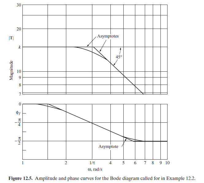
Step 4. The Bode diagram curves for amplitude and phase can now be plotted with calculations based on the expressions for T(ω) and  \phi_{T}(ω) developed in Step 3. The resulting magnitude and phase curves for this first-order system are shown in Fig. 12.5.

In a preliminary system analysis, it is often sufficient to approximate the amplitude and phase curves by use of simple straight-line asymptotes, which are very easily sketched by hand. These straight-line asymptotes are included in Fig. 12.5. The first asymptote for the magnitude curve corresponds to the case in which _ is very small, approaching zero. Using Equation (12.35) for the magnitude as ω→0 yields

\underset{\omega \rightarrow 0}{\lim }\left[\log T(\omega )\right]  =\underset{\omega \rightarrow 0}{\lim }\left(\log \frac{k}{\sqrt{1+\omega ^{2}\tau ^{2}  } } \right) =\log k  .     (12.40)