Known An air compressor rapidly fills a tank having a known volume. The initial state of the air in the tank and the state of the entering air are known.
Find Plot the pressure and temperature of the air within the tank, and plot the air compressor work input, each versus m / m _{1} ranging from 1 to 3.
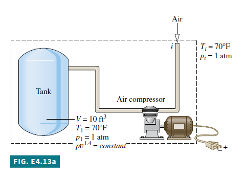
Schematic and Given Data:
Engineering Model
1. The control volume is defined by the dashed line on the accompanying diagram.
2. Because the tank is filled rapidly, \dot{Q}_{ cv } is ignored.
3. Kinetic and potential energy effects are negligible.
4. The state of the air entering the control volume remains constant.
5. The air stored within the air compressor and interconnecting pipes can be ignored.
1 6. The relationship between pressure and specific volume for the air in the tank is p v^{1.4}=\text { constant }.
7. The ideal gas model applies for the air.
Analysis The required plots are developed using Interactive Thermodynamics: IT. The IT program is based on the following
analysis. The pressure p in the tank at time t > 0 is determined from
p v^{1.4}=p_{1} v_{1}^{1.4}
where the corresponding specific volume υ is obtained using the known tank volume V and the mass m in the tank at that time. That is, υ = V/m. The specific volume of the air in the tank initially, v_{1}, is calculated from the ideal gas equation of state and the known initial temperature, T_{1}, \text { and pressure, } p_{1}. That is,
v_{1}=\frac{R T_{1}}{p_{1}}=\frac{\left(\frac{1545 ft \cdot lbf }{28.97 lb \cdot{ }^{\circ} R }\right)\left(530^{\circ} R \right)}{\left(14.7 lbf / in .^{2}\right)}\left|\frac{1 ft ^{2}}{144 in ^{2}}\right|=13.35 \frac{ ft ^{3}}{ lb }
Once the pressure p is known, the corresponding temperature T can be found from the ideal gas equation of state, T = pv/R.
To determine the work, begin with the mass rate balance Eq. 4.2, which reduces for the single-inlet control volume to
\frac{d m_{ cv }}{d t}=\sum_{i} \dot{m}_{i}-\sum_{e} \dot{m}_{e} (4.2)
\frac{d m_{ cv }}{d t}=\dot{m}_{i}
Then, with assumptions 2 and 3, the energy rate balance Eq. 4.15 reduces to
\frac{d E_{ cv }}{d t}=\dot{Q}_{ cv }-\dot{W}_{ cv }+\sum_{i} \dot{m}_{i}\left(h_{i}+\frac{ V _{i}^{2}}{2}+g z_{i}\right)-\sum_{e} \dot{m}_{e}\left(h_{e}+\frac{ V _{e}^{2}}{2}+g z_{e}\right) (4.15)
\frac{d U_{ cv }}{d t}=-\dot{W}_{ cv }+\dot{m}_{i} h_{i}
Combining the mass and energy rate balances and integrating using assumption 4 give
\Delta U_{ cv }=-W_{ cv }+h_{i} \Delta m_{ cv }
Denoting the work input to the compressor by W_{\text {in }}=-W_{ cv } and using assumption 5, this becomes
2 W_{\text {in }}=m u-m_{1} u_{1}-\left(m-m_{1}\right) h_{i} (a)
where m_{1} is the initial amount of air in the tank, determined from
m_{1}=\frac{V}{v_{1}}=\frac{10 ft ^{3}}{13.35 ft ^{3} / lb }=0.75 lb
As a sample calculation to validate the IT program below, consider the case m = 1.5 lb, which corresponds to m / m_{1}=2. The specific volume of the air in the tank at that time is
v=\frac{V}{m}=\frac{10 ft ^{3}}{1.5 lb }=6.67 \frac{ ft ^{3}}{ lb }
The corresponding pressure of the air is
p=p_{1}\left(\frac{v_{1}}{v}\right)^{1.4}=(1 atm )\left(\frac{13.35 ft ^{3} / lb }{6.67 ft ^{3} / lb }\right)^{1.4}
= 2.64 atm
and the corresponding temperature of the air is
T=\frac{p v}{R}=\left(\frac{(2.64 atm )\left(6.67 ft ^{3} / lb \right)}{\left(\frac{1545 ft \cdot lbf }{28.97 lb \cdot{ }^{\circ} R }\right)}\right)\left | \frac{14.7 lbf / in.^{2}}{1 atm } \right | \left |\frac{144 in .^{2}}{1 ft ^{2}} \right |
= 699^{\circ} R \left(239^{\circ} F \right)
Evaluating u_{1}, u, \text { and } h_{i} at the appropriate temperatures from Table A-22E, u_{1}=90.3 Btu / lb , u=119.4 Btu / lb , h_{i}=126.7 Btu/lb. Using Eq. (a), the required work input is
W_{\text {in }}=m u-m_{1} u_{1}-\left(m-m_{1}\right) h_{i}
=(1.5 lb )\left(119.4 \frac{ B tu }{ lb }\right)-(0.75 lb )\left(90.3 \frac{ B tu }{ lb }\right)
-(0.75 lb )\left(126.7 \frac{ Btu }{ lb }\right)
= 16.4 Btu
IT Program Choosing English units from the Units menu, and selecting Air from the Properties menu, the IT program for solving the problem is
Using the Solve button, obtain a solution for the sample case r = m/m_{1} = 2 considered above to validate the program. Good agreement is obtained, as can be verified. Once the program is validated, use the Explore button to vary the ratio m/m1 from 1 to 3 in steps of 0.01. Then, use the Graph button to construct the required plots. The results follow:
We conclude from the first two plots that the pressure and temperature each increase as the tank fills. The work required to fill the tank increases as well. These results are as expected.
1 This pressure-specific volume relationship is in accord with what might be measured. The relationship is also consistent with the uniform state idealization, embodied by Eqs. 4.26 and 4.27.
2 This expression can also be obtained by reducing Eq. 4.28. The details are left as an exercise.
m_{ cv }(t)=V_{ cv }(t) / v(t) (4.26)
U_{ cv }(t)=m_{ cv }(t) u(t) (4.27)
m_{ cv }(t) u(t)-m_{ cv }(0) u(0)=Q_{ cv }-W_{ cv }+h_{i}\left(m_{ cv }(t)-m_{ cv }(0)\right) (4.28)
Skills Developed
Ability to…
• apply the time-dependent mass and energy rate balances to a control volume.
• develop an engineering model.
• retrieve property data for air modeled as an ideal gas.
• solve iteratively and plot the results using IT.
Quick Quiz
As a sample calculation, for the case m = 2.25 lb, evaluate p, in atm. Compare with the value read from the plot of Fig. E4.13b. Ans. 4.67 atm.