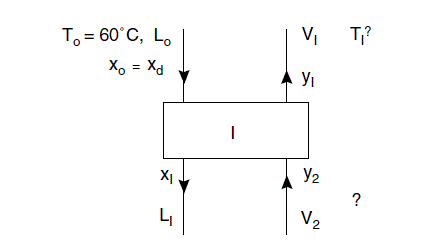
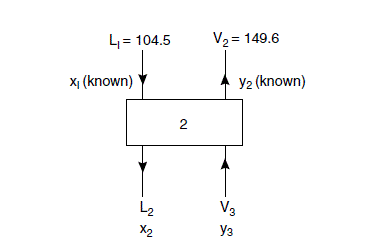
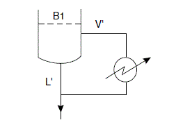
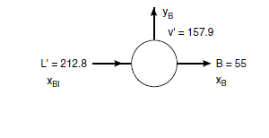
Only sufficient trial calculations will be made to illustrate the method used. Basis 100 mol feed.
Estimation of dew and bubble points
\text { Bubble point } \sum y_{i}=\sum K_{i} x_{i}=1.0 (11.5a)
\text { Dew point } \sum x_{i}=\sum \frac{y_{i}}{K_{i}}=1.0 (11.5b)
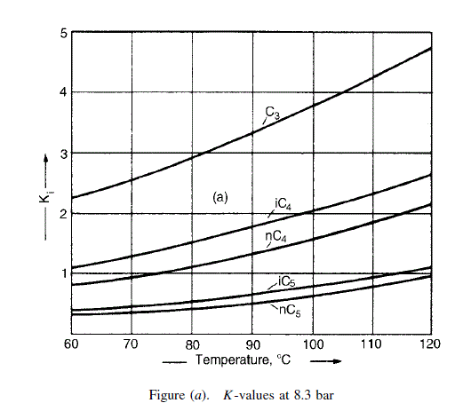
The K values, taken from the De Priester charts (Chapter 8), are plotted in Figure (a) for easy interpolation.
To estimate the dew and bubble points, assume that nothing heavier than the heavy key appears in the tops, and nothing lighter than the light key in the bottoms.
|
d |
x_{d} |
b |
x_{b} |
| C _{3} |
5 |
0.11 |
0 |
_ |
| C _{4} |
15 |
0.33 |
0 |
_ |
| nC _{4} |
24 |
0.54 |
1 |
0.02 |
| iC _{5} |
1 |
0.02 |
19 |
0.34 |
| nC _{5} |
0 |
_ |
35 |
0.64 |
|
45 |
|
55 |
|
Bubble-point calculation, bottoms
|
x_{b} |
\text { Try } 100^{\circ} C |
\text { Try } 120^{\circ} C |
| K_{i} |
K_{i} x_{i} |
K_{i} |
K_{i} x_{i} |
| C _{3} |
_ |
_ |
_ |
_ |
_ |
| iC _{4} |
_ |
_ |
_ |
_ |
_ |
| nC _{4} |
0.02 |
1085 |
0.04 |
2.1 |
0.04 |
| iC _{5} |
0.34 |
0.94 |
0.32 |
1.1 |
0.37 |
| nC _{5} |
0.64 |
0.82 |
0.52 |
0.96 |
0.61 |
|
\Sigma K_{i} x_{i}=0.88 temp. too low |
1.02 close enough |
Bubble-point calculation, feed (liquid feed)
|
x_{d} |
\text { Try } 70^{\circ} C |
\text { Try } 60^{\circ} C |
| K_{i} |
y_{i} / K_{i} |
K_{i} |
y_{i} / K_{i} |
| C _{3} |
0.11 |
2.6 |
0.04 |
2.20 |
0.24 |
| iC _{4} |
0.33 |
1.3 |
0.25 |
1.06 |
0.35 |
| nC _{4} |
0.54 |
0.9 |
0.60 |
0.77 |
0.42 |
| iC _{5} |
0.02 |
0.46 |
0.04 |
0.36 |
0.01 |
| nC _{5} |
_ |
_ |
_ |
_ |
_ |
|
\Sigma y_{i} / K_{i}=0.94 temp. too high |
1.02 close enough |
Bubble-point calculation, feed (liquid feed)
|
x_{f} |
\text { Try } 80^{\circ} C |
\text { Try } 90^{\circ} C |
\text { Try } 85^{\circ} C |
| K_{i} |
x_{i} K_{i} |
K_{i} |
x_{i} K_{i} |
K_{i} |
x_{i} K_{i} |
| C _{3} |
0.05 |
2.9 |
0.15 |
3.4 |
0.17 |
3.15 |
0.16 |
| iC _{4} |
0.15 |
1.5 |
0.23 |
1.8 |
0.27 |
1.66 |
0.25 |
| nC _{4} |
0.25 |
1.1 |
0.28 |
1.3 |
0.33 |
1.21 |
0.30 |
| iC _{5} |
0.20 |
0.5 |
0.11 |
0.66 |
0.13 |
0.60 |
0.12 |
| nC _{5} |
0.35 |
0.47 |
0.16 |
0.56 |
0.20 |
0.48 |
0.17 |
|
0.93 temp. too low |
1.10 temp. too high |
1.00 satisfactory |
Stage-by-stage calculations
Top down calculations, assume total condensation with no subcooling
y_{1}=x_{d}=x_{0}
It is necessary to estimate the composition of the “non-keys” so that they can be included in the stage calculations. As a first trial the following values will be assumed:
|
X _{d} |
| C _{3} |
0.10 |
5 |
| iC _{4} |
0.33 |
15 |
| nC _{4} |
0.54 |
24 |
| iC _{5} |
0.02 |
1 |
| nC _{5} |
0.001 |
0.1 |
|
45.1 |
In each stage calculation it will necessary to estimate the stage temperatures to determine the K values and liquid and vapour enthalpies. The temperature range from top to bottom of the column will be approximately 120 – 60 = 5^{\circ} C. An approximate calculation (Example 11.7) has shown that around fourteen ideal stages will be needed; so the temperature change from stage to stage can be expected to be around 4 to 5^{\circ} C.
Stage 1
L_{0}=R \times D=2.5 \times 45.1=112.8
V_{1}=(R+1) D=3.5 \times 45.1=157.9
Estimation of stage temperature and outlet liquid composition (x1)
|
y_{1} |
\text { Try } T_{1}=66^{\circ} C |
\text { Try } T_{1}=65^{\circ} C |
|
| K_{i} |
y_{i} / K_{i} |
K_{i} |
y_{i} / K_{i} |
x_{1}=y_{i} / K_{i} Normalised |
| C _{3} |
0.1 |
2.4 |
0.042 |
2.36 |
0.042 |
0.042 |
| iC _{4} |
0.33 |
1.2 |
0.275 |
1.19 |
0.277 |
0.278 |
| nC _{4} |
0.54 |
0.88 |
0.614 |
0.86 |
0.628 |
0.629 |
| iC _{5} |
0.02 |
0.42 |
0.048 |
0.42 |
0.048 |
0.048 |
| nC _{5} |
0.001 |
0.32 |
0.003 |
0.32 |
0.003 |
0.003 |
|
\Sigma y_{i} / K_{i}=0.982 too low |
0.998 close enough |
|
Summary of stage equations
L_{0}+V_{2}=L_{1}+V_{1} (i)
L_{0} x_{0}+V_{2} y_{2}=L_{1} x_{1}+V_{1} y_{1} (ii)
h_{0} L_{0}+H_{2} V_{2}=h_{1} L_{1}+H_{1} V_{1} (iii)
h=f(x, T) (iv)
H=f(x, T) (v)
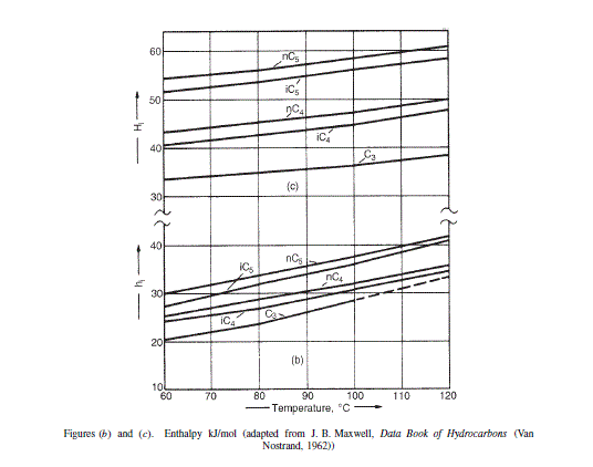
The enthalpy relationship is plotted in Figures (b) and (c).
y_{i}=K_{i} x_{i} (vi)
Before a heat balance can be made to estimate L_{1} \text { and } V_{2}, an estimate of y_{2} \text { and } T_{2} is needed. y_{2} is dependent on the liquid and vapour flows, so as a first trial assume that
these are constant and equal to L_{0} \text { and } V_{1}; then, from equations (i) and (ii),
y_{2}=\left(\frac{L_{0}}{V_{1}}\right)\left(x_{1}-x_{0}\right)+y_{1}
\frac{L_{0}}{V_{1}}=\frac{112.8}{157.9}=0.71
|
x_{1} |
x_{0} |
y_{2}=0.71\left(x_{1}-x_{0}\right)+y_{1} |
y_{2} Normalised |
| C _{3} |
0.042 |
0.10 |
0.057 |
0.057 |
| iC _{4} |
0.278 |
0.33 |
0.294 |
0.292 |
| nC _{4} |
0.629 |
0.54 |
0.604 |
0.600 |
| iC _{5} |
0.048 |
0.02 |
0.041 |
0.041 |
| nC _{5} |
0.003 |
0.001 |
0.013 |
0.013 |
|
1.009 close enough |
Enthalpy data from Figures (b) and (c) J/mol
|
h_{0}\left(T_{0}=60^{\circ} C \right) |
h_{1}\left(T_{1}=65^{\circ} C \right) |
| x_{0} |
h_{i} |
h_{j} x_{i} |
x_{1} |
h_{i} |
h_{j} x_{i} |
| C _{3} |
0.10 |
20,400 |
2040 |
0.042 |
21,000 |
882 |
| iC _{4} |
0.33 |
23,400 |
7722 |
0.278 |
24,900 |
6897 |
| nC _{4} |
0.54 |
25,200 |
13,608 |
0.629 |
26,000 |
16,328 |
| iC _{5} |
0.02 |
27,500 |
550 |
0.048 |
28,400 |
1363 |
| nC _{5} |
0.001 |
30,000 |
30 |
0.003 |
30,700 |
92 |
|
h_{0}=23,950 |
h_{1}=25,562 |
|
H_{1}\left(T_{1}=65^{\circ} C \right) |
h_{1}\left(T_{1}=65^{\circ} C \right) |
| v_{1} |
H_{i} |
H_{i} y_{i} |
y_{2} |
H_{i} |
H_{i} y_{i} |
| C _{3} |
0.10 |
34,000 |
3400 |
0.057 |
34,800 |
1984 |
| iC _{4} |
0.33 |
41,000 |
13,530 |
0.292 |
41,300 |
12,142 |
| nC _{4} |
0.54 |
43,700 |
23,498 |
0.600 |
44,200 |
26,697 |
| iC _{5} |
0.02 |
52,000 |
1040 |
0.041 |
52,500 |
2153 |
| nC _{5} |
0.001 |
54,800 |
55 |
0.013 |
55,000 |
715 |
|
H_{1}=41,623 |
H_{2}=43,691 |
Energy balance (equation iii)
23,950 \times 112.8+43,691 V_{2}=25,562 L_{1}+41,623 \times 157.9
43,691 V_{2}=255,626 L_{1}+3,870,712
Material balance (equation i)
112.8+V_{2}=L_{1}+157.9
substituting
43,691\left(L_{1}+45.1\right)=25,562 L_{1}+3,870,712
L_{1}=104.8
V_{2}=104.8+45.1=149.9
\frac{L_{1}}{V_{2}}=0.70
Could revise calculated values for y_{2} \text { but } L_{1} / V_{2} is close enough to assumed value of 0.71, so there would be no significant difference from first estimate.
Stage 2
Estimation of stage temperature and outlet liquid composition (x2).
|
y_{2} |
T_{2}=70^{\circ} C \text { (use assumed value as first trial) } |
| K_{i} |
x_{2}=y_{2} / K_{i} |
x_{2} Normalised |
| C _{3} |
0.057 |
2.55 |
0.022 |
0.022 |
| iC _{4} |
0.292 |
1.30 |
0.226 |
0.222 |
| nC _{4} |
0.600 |
0.94 |
0.643 |
0.630 |
| iC _{5} |
0.041 |
0.43 |
0.095 |
0.093 |
| nC _{5} |
0.013 |
0.38 |
0.034 |
0.033 |
|
1.020 close enough to 1.0 |
y_{3}=\frac{L}{V}\left(x_{2}-x_{1}\right)+y_{2}
\text { As a first trial take } L / V \text { as } L_{1} / V_{1}=0.70
|
x_{2} |
x_{1} |
y_{3}=0.70\left(x_{2}-x_{1}\right)+y_{2} |
y_{3} Normalised |
| C _{3} |
0.02 |
0.042 |
0.044 |
0.043 |
| iC _{4} |
0.222 |
0.277 |
0.256 |
0.251 |
| nC _{4} |
0.630 |
0.628 |
0.0613 |
0.601 |
| iC _{5} |
0.093 |
0.048 |
0.072 |
0.072 |
| nC _{5} |
0.033 |
0.003 |
0.035 |
0.034 |
|
|
|
1.020 |
|
Enthalpy data from Figures (b) and (c)
|
h_{2}\left(T_{2}=70^{\circ} C \right) |
H_{3}\left(T_{3}=75^{\circ} C \text { assumed }\right) |
| x_{2} |
h_{i} |
h_{i} x_{2} |
y_{3} |
H_{i} |
H_{i} y_{3} |
| C _{3} |
0.022 |
21,900 |
482 |
0.043 |
34,600 |
1488 |
| iC _{4} |
0.222 |
25,300 |
5617 |
0.251 |
41,800 |
10,492 |
| nC _{4} |
0.630 |
27,000 |
17,010 |
0.601 |
44,700 |
26,865 |
| iC _{5} |
0.093 |
29,500 |
2744 |
0.072 |
53,000 |
3816 |
| nC _{5} |
0.033 |
31,600 |
1043 |
0.035 |
55,400 |
1939 |
|
h_{2}=26,896 |
H_{3}=44,600 |
Energy balance
25,562 \times 104.8+44,600 V_{3}=4369 \times 149.9+26,896 L_{2}
Material balance
104.8+V_{3}=149.9+L_{2}
L_{2}=105.0
V_{3}=150.1
\frac{L_{2}}{V_{3}}=0.70 \text { checks with assumed value. }
Stage 3
As the calculated liquid and vapour flows are not changing much from stage to stage the calculation will be continued with the value of L/V taken as constant at 0.7.
|
\text { Try } T_{3}=75^{\circ} C \text { (assumed value) } |
y_{4}=0.7\left(x_{3}-x_{2}\right)+y_{3} |
| K_{i} |
x_{3}=y_{3} / K_{i} |
Normalised |
| C _{3} |
2.71 |
0.016 |
0.015 |
0.38 |
| iC _{4} |
1.40 |
0.183 |
0.177 |
0.217 |
| nC _{4} |
1.02 |
0.601 |
0.580 |
0.570 |
| iC _{5} |
0.50 |
0.144 |
0.139 |
0.104 |
| nC _{5} |
0.38 |
0.092 |
0.089 |
0.074 |
|
1.036 Close enough |
1.003 |
|
\text { Try } T_{4}=81^{\circ} C |
y_{5}=0.7\left(x_{4}-x_{3}\right)+y_{4} |
| K_{i} |
x_{4}=y_{4} / K_{i} |
Normalised |
| C _{3} |
2.95 |
0.013 |
0.013 |
0.39 |
| iC _{4} |
1.55 |
0.140 |
0.139 |
0.199 |
| nC _{4} |
1.13 |
0.504 |
0.501 |
0.515 |
| iC _{5} |
0.55 |
0.189 |
0.188 |
0.137 |
| nC _{5} |
0.46 |
0.161 |
0.166 |
0.118 |
|
1.007 |
Close enough |
1.008 |
Stage 5
|
\text { Try } T_{5}=85^{\circ} C |
y_{6}=0.7\left(x_{5}-x_{4}\right)+y_{5} |
| K_{i} |
x_{5} |
Normalised |
| C _{3} |
3.12 |
0.013 |
0.012 |
0.038 |
| iC _{4} |
1.66 |
0.120 |
0.115 |
0.179 |
| nC _{4} |
1.20 |
0.430 |
0.410 |
0.450 |
| iC _{5} |
0.60 |
0.228 |
0.218 |
0.159 |
| nC _{5} |
46 |
0.257 |
0.245 |
0.192 |
|
1.048 |
Close enough |
1.018 |
Stage 6
|
\text { Try } T_{6}=90^{\circ} C |
K_{i} |
\text { Try } T_{6}=92^{\circ} C |
x_{7} |
| K_{i} |
x_{6} |
x_{6} |
Normalised |
| C _{3} |
3.35 |
0.011 |
3.45 |
0.011 |
0.011 |
0.037 |
| iC _{4} |
1.80 |
0.099 |
1.85 |
0.097 |
0.095 |
0.166 |
| nC _{4} |
1.32 |
0.341 |
1.38 |
0.376 |
0.318 |
0.386 |
| iC _{5} |
0.65 |
0.245 |
0.69 |
0.230 |
0.224 |
0.163 |
| nC _{5} |
0.51 |
0.376 |
0.53 |
0.362 |
0.350 |
0.268 |
|
1.072 too low |
1.026 close enough |
1.02 |
\text { Note: ratio of } LK \text { to } HK \text { in liquid from this stage }=\frac{0.386}{0.163}=2.37
Stage 7
|
\text { Try } T_{6}=97^{\circ} C |
| K_{i} |
x_{7} |
Normalised |
| C _{3} |
3.65 |
0.010 |
0.010 |
| iC _{4} |
1.98 |
0.084 |
0.083 |
| nC _{4} |
1.52 |
0.254 |
0.251 |
| iC _{5} |
0.75 |
0.217 |
0.214 |
| nC _{5} |
0.60 |
0.447 |
0.442 |
|
1.012 |
|
\text { ratio } \frac{ LK }{ HK }=\frac{0.251}{0.214}=1.17
This is just below the ratio in the feed
=\frac{25}{20}=1.25
So, the feed would be introduced at this stage.
But the composition of the non-key components on the plate does not match the feed composition.
|
x_{f} |
x_{7} |
| C _{3} |
0.05 |
0.10 |
| iC _{4} |
0.15 |
0.084 |
| nC _{4} |
0.25 |
0.254 |
| iC _{5} |
0.20 |
0.217 |
| nC _{5} |
0.35 |
0.447 |
So it would be necessary to adjust the assumed top composition and repeat the calculation.
Bottom-up calculation
To illustrate the procedure the calculation will be shown for the reboiler and bottom stage, assuming constant molar overflow.
With the feed at its boiling point and constant molar overflow the base flows can be calculated as follows:
V^{\prime}=V_{0}=157.9
L^{\prime}=L_{0}+ FEED =112.8+100=212.8
\frac{V^{\prime}}{L^{\prime}}=\frac{157.9}{212.8}=0.74
It will be necessary to estimate the concentration of the non-key components in the bottom product; as a first trial take:
| C _{3} |
iC _{4} |
nC _{4} |
iC _{5} |
nC _{5} |
| 0.001 |
0.001 |
0.02 |
0.34 |
0.64 |
Reboiler
Check bubble-point estimate of 120^{\circ} C
|
x_{B} |
\text { Try } 120^{\circ} C |
\text { Try } 118^{\circ} C |
| K_{i} |
y_{B}=K_{i} x_{B} |
K_{i} |
y_{B} |
| C _{3} |
0.001 |
4.73 |
0.005 |
4.60 |
0.005 |
| iC _{4} |
0.001 |
2.65 |
0.003 |
2.58 |
0.003 |
| nC _{4} |
0.02 |
2.10 |
0.042 |
2.03 |
0.041 |
| iC _{5} |
0.34 |
1.10 |
0.374 |
1.06 |
0.360 |
| nC _{5} |
0.64 |
0.96 |
0.614 |
0.92 |
0.589 |
|
1.038 too high |
0.998 close enough |
Material balance:
x_{B 1} L^{\prime}=y_{B} V^{\prime}+x_{B} B
x_{B 1}=\frac{V^{\prime}}{L^{\prime}} y_{B}+\frac{B}{L^{\prime}} x_{B}
x_{B 1}=\frac{157.9}{212.8} y_{B}+\frac{55}{212.8} x_{B} =0.74 y_{B}+0.26 x_{B}
Stage 1 from base (B1)
|
x_{B} |
y_{B} |
x_{B 1} |
x_{B 2}=0.74\left(y_{1 B}-y_{B}\right)+x_{1 B} |
| C _{3} |
0.001 |
0.005 |
0.004 |
0.014 |
| iC _{4} |
0.001 |
0.003 |
0.002 |
0.036 |
| nC _{4} |
0.02 |
0.041 |
0.020 |
0.019 |
| iC _{5} |
0.34 |
0.361 |
0.356 |
0.357 |
| nC _{5} |
0.64 |
0.590 |
0.603 |
0.559 |
|
0.985 |
The calculation is continued stage-by-stage up the column to the feed point (stage 7 from the top). If the vapour composition at the feed point does not mesh with the top-down calculation, the assumed concentration of the non-keys in the bottom product is adjusted and the calculations repeated.
