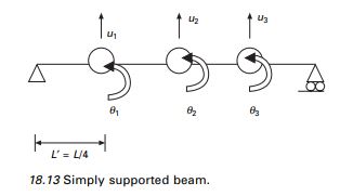
Question 18.7: Figure 18.13 shows a mass-less simply suported beam with thr......
Figure 18.13 shows a mass-less simply suported beam with three lumped masses and the following properties: L = 3.81 m, m = 33665 kg, E = 207.15 GPa.
We are interested in studying the dynamic response of the beam to F(t) = Ff(t) where < F >=<1 0 0>.
(a) Determine the modal expansion of vector {F} that defines the spatial distribution of force.
(b) For the bending moment M_1 at the location of U_1 degrees of freedom determine the modal static response
M_1^{s t}=\sum\limits_{n-1}^N M_{1 n}^{s t}
(c) Calculate and tabulate modal contribution factors their cumulative values for various numbers of modes included J = 1, 2, 3 and the error e_j for static response. Comment on how the relative values of modal contribution factors and the error e_j are influenced by spatial distribution of forces.
(d) Determine the peak value of (M_{1n})_0 modal response due to F(t)
p(t)=\left\{\begin{array}{cl}p_o \sin \pi t / t d & t \leq t d \\0 & t \geq t d\end{array}\right\}
Assume t_d = 0.598~ s which is the same as T_{1}.
The distribution of the pulse t{d} = T_{1} the fundamental period of the system. For the shock spectrum of half cycle sine wave R_d = 1.73, 1.14 and 1.06 for T_1/t_d = 1; T_2/t_d = 0.252; T_3/t_d = 0.119 respectively. It will be convenient to organize the computation in a table with following headings:
n, T_n / t_d, R_{d n}, \bar{M}_{1 n} \text { and}\left[\left(M_{1 n}\right)_0 /\left(p_0 M_1^{st}\right)\right](e) Comment on how the peak modal response determined in part (d) depend on modal static response, modal contributed factor \bar{M}_{1 n} and R_{d n} and S.
(f) Is it possible to determine the peak value of the total (considering all modes) response from peak modal response? Justify your answer.
E = 207.15 GPa
m = 33 665 kg
L = 3.81 m
I=4.1623 \times 10^7~ mm ^4| Table 18.3 Dynamic base shear calculation | ||||
| Mode | \omega_n | \bar{R}=\frac{U_{1i}}{U_1^{\text {st }}} | R_d=\frac{1}{1~-~\left(\frac{\omega}{\omega_i}\right)^2} | \bar{\gamma}=\bar{R} ~R_d |
| 1 | 28.5 | \frac{0.0095}{0.0079}=1.21 | 2.28 | 2.758 |
| 2 | 69 | \frac{-0.0016}{0.0079}=-0.211 | 1.106 | –0.232 |

Learn more on how do we answer questions.
Step 1
U_M^{ T }=<U_1 ~U_2 ~U_3>; U_S^{ T }=<\theta_1~ \theta_2~ \theta_3>
Step 2 Mass matrix
m=\left[\begin{array}{lll}33665 & & \\& 33665 & \\& & 33665\end{array}\right]
Step 3 Determine stiffness matrix (sym)
K=\frac{E I}{L^{\prime 3}}\left[\begin{array}{ccc|ccc}7 L^{\prime 2} & 2 L^{\prime 2} & 0 & 3 L^{\prime} & -6L^{\prime} & 0 \\& 8 L^{\prime 2} & 2 L^{\prime 2} & 6 L^{\prime} & 0 & -6 L^{\prime} \\& & 7 L^{\prime 2} & 0 & 6 L^{\prime} & -3 L^{\prime} \\& K s s & & K S M & & \\\hline & & & 15 & -12 & 0 \\& & & & 24 & -12 \\& & & & & 15\\& K ms && K mm & \end{array}\right]
Using the static condensation procedure the modified stiffness matrix for the master degree of freedom can be written as
\frac{E I}{L^{\prime 3}}\left[\begin{array}{ccc}9.8501 & -9.4283 & 3.864 \\& 13.713 & -9.4283 \\\text { sym } & & 9.8501\end{array}\right]
or
Step 4 Determine lateral stiffness
=\frac{E I}{L^3}\left[\begin{array}{ccc}630.86 & -603.43 & 246.86 \\& 877.71 & -603.43 \\& &630.86\end{array}\right]
\frac{E I}{L^3}=\frac{207.15~ \times ~10^9 ~\times~ 4.1623~\times ~10^7}{10^{12}~ \times~ 3.81^3}
= 155 899.02
K=10^5\left[\begin{array}{ccc}983.5 & -940.74 & 384.45 \\& 1368.34 & -940.74 \\\text { Syn } & & 983.5\end{array}\right]
Step 5 Determine natural frequencies solving using the MATHEMATICA package
\omega_1=10.589 ; \omega_2=42.1824, \omega_3=89.55~ rad / s
E V=\left[\begin{array}{ccc}0.50 & 0.707 & 0.50 \\0.707 & 0 & -0.707 \\0.50 & -0.707 & 0.50\end{array}\right]
Normalized eigenvector =\phi^{ T } m \varphi=I
where
\varphi=\left[\begin{array}{ccc}0.0027 &0.00385 & 0.0027 \\0.00385 & 0 & -0.00385 \\0.0027 & -0.00385 & 0.0027\end{array}\right]
The mode shapes are shown in Fig. 18.14.
Step 6 Determine modal expansion F
F=\sum\limits_{n=1}^3 F_n
=\Sigma~ \Gamma_n m \phi_n~ \text { where }~\Gamma_n=\phi_n^{ T }~ F
\Gamma=\left\{\begin{array}{c}0.0027 \\0.00385 \\0.0027\end{array}\right\}
F_1=\Gamma_1 m \phi_1
The modal expansion of F is shown graphically in Fig. 18.15 and tabulated in Table 18.4.
Step 7 Determine modal static response as shown in Fig. 18.16. The value of moments due to forces F is determined by the linear combination to the above three load cases.
The resultants are as given in Table 18.5.
Next we can determine
M_1^{s t}=\frac{3 L}{16}
= 0.1875L
We have demonstrated
\sum\limits_{n=1}^3 ~M_{1 n}^{s t}=M_1^{s t}
Step 8 Determine modal contribution factors, their cumulative values and error.
The modal contribution factors and error are given in Table 18.6
In the above the modal contribution factor is largest for first mode and progressively decreases for the second and third modes.
Step 9 Determine response to the half cycle sine pulse. The peak modal response equation is specialized for R = M_{1} to obtain (see Table 18.7)
\left(M_{1 n}\right)_0=p_0 M_1^{s t}~ \bar{M}_{1 n} ~R_{d n}
Step 10 Comments
• For the given force, the modal response decreases for higher modes. The decrease is more rapid because of R_{dn}. It also decreases with mode n.
• The peak value of the total response cannot be determined from the peak modal response because the modal peaks occur at different time instants. Square root of sum of squares (SRSS) and complete quadratic combination (CQC) do not apply to pulse excitations.
| Table 18.4 Modal contribution of excitation vectors |
|||
| F | F_1 | F_2 | F_3 |
| 1 | 0.25 | 0.5 | 0.25 |
| 0 | 0.35 | 0 | –0.35 |
| 0 | 0.25 | –0.5 | 0.25 |
| Table 18.5 Calculation of moment at 1 | |
| Mode | M_{1 n}^{s t} \text { due to } F |
| 1 | 0.25 \times \frac{3 L}{16}+0.35 \times \frac{L}{8}+0.25\frac{L}{16}=0.10672 ~L |
| 2 | 0.5 \times \frac{3 L}{16}-0.5 \frac{L}{16}=0.0625 ~L |
| 3 | 0.25 \times \frac{3 L}{16}-0.35 \frac{L}{8}+0.25 \frac{L}{16}=0.0183 ~L |
| \sum\limits_{n=1}^3 M_{1 n}^{s t} | 0.1875 × L = 0.1875 × 3.81 L |
| = 0.7143 N m | |
| Table 18.6 Modal contribution and error | |||
| Mode n_1 or no. of modes J | Due to F \bar{M}_{1 n} | \sum\limits_{n=1}^J M_1 n | e |
| 1 | \frac{0.1067}{0.1875}=0.5691 | 0.5691 | 0.4309 |
| 2 | \frac{0.625}{0.1875}=0.333 | 0.9024 | 0.0976 |
| 3 | \frac{0.0183}{0.1875}=0.0976 | 1.0 | 0 |
| Table 18.7 Peak modal response | ||||
| Mode n | Spectral values T_{n}/t_{d} |
R_{dn} | \bar{M}_1 n | \begin{aligned}& M _{1 n} \times R_{d n} \\&\left(M_{1n}\right)_0 /\left(p_0M_1^{st}\right)\end{aligned} |
| 1 | 1 | 1.73 | 0.5691 | 0.985 |
| 2 | 0.252 | 1.14 | 0.333 | 0.379 |
| 3 | 0.119 | 1.06 | 0.0976 | 0.103 |


