Question 20.3: Figure P.20.3 shows the cross-section of a single-cell, thin......
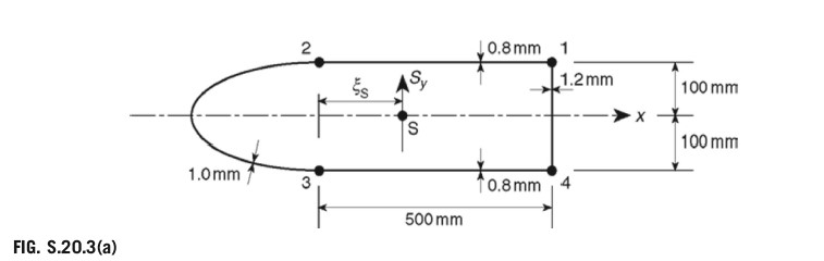
Figure P.20.3 shows the cross-section of a single-cell, thin-walled beam with a horizontal axis of symmetry. The direct stresses are carried by the booms B_{1} to B_{4}, while the walls are effective only in carrying shear stresses. Assuming that the basic theory of bending is applicable, calculate the position of the shear center S. The shear modulus G is the same for all walls:
Cell area = 135, 000 mm²; Boom areas: B_{1}=B_{4}=450\;\mathrm{mm}^{2},\;\;B_{2}=B_{3}=550\;\mathrm{mm}^{2}
\begin{array}{l l l}{{\mathrm{Wall}}}&{{\mathrm{~{Length~(mm)}}}}&{{\mathrm{~Thickness~(mm)}}}\\ {{\mathrm{~12,~34~}}}&{{\mathrm{~500~}}}&{{\mathrm{~0.8~}}}\\ {{\mathrm{~23~}}}&{{\mathrm{~580~}}}&{{\mathrm{~1.0~}}}\\ {{\mathrm{~41~}}}&{{\mathrm{~200~}}}&{{\mathrm{~1.2~}}}\end{array}Answer: 197.2 mm to the right of the vertical through booms 2 and 3

Learn more on how do we answer questions.
The shear center, S, lies on the horizontal axis of symmetry, the x axis. Therefore apply an arbitrary shear load, S_{y}, through S (Fig. S.20.3(a)). The internal shear flow distribution is given by Eq. (20.11), which, since I_{x y}=0,\,S_{x}=0,\,{\mathrm{and}}\,\,t_{\mathrm{D}}=0, simplifies to
q_{s}=-\left({\frac{S_{x}I_{x x}-S_{y}I_{x y}}{I_{x x}I_{y y}-I_{x y}^{2}}}\right) \left(\int_{0}^{s}t_{\mathrm{D}}x\,\mathrm{d}s+\sum\limits_{r=1}^{n}B_{r}x_{r}\right) -\left(\frac{S_{y}I_{y y}-S_{x}I_{x y}}{I_{x x}I_{y y}-I_{x y}^{2}}\right) \left(\int_{0}^{s}t_{\mathrm{DJ}}\,\mathrm{d}s+\sum\limits_{r=1}^{n}B_{r}y_{r}\right)+q_{s,0} (20.11)
q_{s}=-{\frac{S_{y}}{I_{x x}}}\sum\limits_{r=1}^{n}B_{r}y_{r}+q_{s,0} (i)
in which
I_{x x}=2\times450\times100^{2}+2\times550\times100^{2}=20\times10^{6}{\mathrm{mm}}^{4}Equation (i) then becomes
q_{s}=-0.5\times10^{-7}S_{y}\sum_{r=1}^{n}B_{r}y_{r}+q_{s,0} (ii)
The first term on the right-hand side of Eq. (ii) is the q_{b} distribution (see Eq. (17.16)). To determine q_{b}, ‘cut’ the section in the wall 23. Then
q_{s}=q_{b}+q_{s,0} (17.16)
The value of shear flow at the ‘cut’ is obtained using Eq. (17.28), which, since G= constant, becomes
q_{s,0}=-{\frac{\oint q_{b}\;\mathrm{d}s}{\oint\mathrm{d}s}} (17.28)
q_{s,0}=-{\frac{\oint(q_{\mathrm{b}}/t)\mathrm{d}s}{\oint\mathrm{d}s/t}} (iii)
In Eq. (iii),
\oint{\frac{ds}{t}}={\frac{580}{1.0}}+2\times{\frac{500}{0.8}}+{\frac{200}{1.2}}=1996.7Then, from Eq. (iii) and the above q_{b} distribution,
q_{s,0}=-{\frac{S_{y}}{1996.7}}\!\left(2\times{\frac{2.75\times10^{-3}\times500}{0.8}}+{\frac{5.0\times10^{-3}\times200}{1.2}}\right)i.e.,
q_{s,0}=-2.14\times10^{-3}S_{y}The complete shear flow distribution is shown in Fig. S.20.3(b).
Now taking moments about O in Fig. S.20.3(b) and using the result of Eq. (20.10),
M_{q}=2A q_{12} (20.10)
S_{y}\xi_{S}=2\times0.61\times10^{-3}S_{y}\times500\times100+2.86\times10^{-3}S_{y}\times200\times500 -2.14\times10^{-3}S_{y}\times2(13500-500\times200)which gives
\xi_{8}=197.2\,{\mathrm{mm}}