Question 6.7.Q1: The following data are provided in Table 6.15: mass radiatio......

(a) Radiation yield Y\left[\left(E_K\right)_0\right] of an electron with initial kinetic energy \left(E_K\right)_0 striking an absorber is defined as that fraction of the initial kinetic energy \left(E_K\right)_0 that is emitted as bremsstrahlung radiation with energy E_{rad} through the slowing down process of the electron in the absorber.

For a heavy charged particle the radiation yield Y\left[\left(E_K\right)_0\right] is zero; however, for light CPs, such as electron and positron, Y\left[\left(E_{\mathrm{K}}\right)_0\right] \neq 0 and can be determined from stopping power data as follows

Y\left[\left(E_{\mathrm{K}}\right)_0\right]=\frac{\int_0^{\left(E_{\mathrm{K}}\right)_0} \frac{S_{\mathrm{rad}}\left(E_{\mathrm{K}}\right)}{S_{\mathrm{tot}}\left(E_{\mathrm{K}}\right)} \mathrm{d} E_{\mathrm{K}}}{\int_0^{\left(E_{\mathrm{K}}\right)_0} \mathrm{~d} E_{\mathrm{K}}}=\frac{1}{\left(E_{\mathrm{K}}\right)_0} \int_0^{\left(E_{\mathrm{K}}\right)_0} \frac{S_{\mathrm{rad}}\left(E_{\mathrm{K}}\right)}{S_{\mathrm{tot}}\left(E_{\mathrm{K}}\right)} \mathrm{d} E_{\mathrm{K}}        (6.104)

Since the ratio S_{\mathrm{rad}}\left(E_{\mathrm{K}}\right) / S_{\mathrm{tot}}\left(E_{\mathrm{K}}\right) is generally not available in an analytical form, the integration in (6.104) is replaced with a numerical summation of S_{\mathrm{rad}} E_{\mathrm{K}} / S_{\text {tot }}\left(E_{\mathrm{K}}\right) using a suitable E_K \text { interval } \Delta E_{\mathrm{K}}.

Y\left[\left(E_{\mathrm{K}}\right)_0\right]=\frac{1}{\left(E_{\mathrm{K}}\right)_0} \int_0^{\left(E_{\mathrm{K}}\right)_0} \frac{S_{\mathrm{rad}}\left(E_{\mathrm{K}}\right)}{S_{\mathrm{tot}}\left(E_{\mathrm{K}}\right)} \mathrm{d} E_{\mathrm{K}}=\frac{1}{\left(E_{\mathrm{K}}\right)_0} \sum_{i=1}^n \overline{\left(\frac{S_{\mathrm{rad}}\left(E_{\mathrm{K}}\right)}{S_{\mathrm{tot}}\left(E_{\mathrm{K}}\right)}\right)_i} \Delta E_{\mathrm{K}},         (6.105)

where \overline{\left(S_{\mathrm{rad}}\left(E_{\mathrm{K}}\right) / S_{\mathrm{tot}}\left(E_{\mathrm{K}}\right)\right)_i} stands for the average value of \left(S_{\mathrm{rad}}\left(E_{\mathrm{K}}\right) / S_{\mathrm{tot}}\left(E_{\mathrm{K}}\right)\right)_i for the interval i and  \overline{\left(S_{\mathrm{rad}}\left(E_{\mathrm{K}}\right) / S_{\text {tot }}\left(E_{\mathrm{K}}\right)\right)_i} \Delta E_{\mathrm{K}} represents the area of interval i in the summation procedure.
To calculate Y\left[\left(E_K\right)_0\right] numerically we use the S_{rad}/S_{tot} data provided in column (6) of Table 6.15, and for practical reasons we choose a relatively wide kinetic energy interval \Delta E_K of 0.5 MeV for the summation. When a computer is used for this purpose, a much narrower interval would be chosen; however, for our proof of principle a manual calculation with an interval \Delta E_K = 0.5 MeV is adequate. Thus, for initial kinetic energy \left(E_K\right)_0 = 4 MeV we will have 8 energy intervals at 0.5 MeV each and, for convenience, we choose E_K = 0 for start of the first interval.
Results of our numerical integration in determination of Y\left[\left(E_K\right)_0\right]\ for\ \left(E_K\right)_0 = 4 MeV are summarized in Table 6.16 and the intervals for the numerical integration are also displayed in Fig. 6.21. Based on data displayed in column (6) of Table 6.16 we now determine Y\left[\left(E_{\mathrm{K}}\right)_0\right] \text { for }\left(E_{\mathrm{K}}\right)_0=4 \mathrm{MeV} as follows

Y\left[\left(E_{\mathrm{K}}\right)_0\right]==\frac{1}{\left(E_{\mathrm{K}}\right)_0} \sum_{i=1}^{n=8} \overline{\left(\frac{S_{\mathrm{rad}}\left(E_{\mathrm{K}}\right)}{S_{\mathrm{tot}}\left(E_{\mathrm{K}}\right)}\right)_i} \Delta E_{\mathrm{K}}=\frac{1}{4  \mathrm{MeV}} \times 0.7002  \mathrm{MeV}=0.175        (6.106)

indicating that 17.5 % of the 4 MeV incident electron kinetic energy is transformed into bremsstrahlung photons. It is noteworthy that our result for Y\left[4\ MeV \right] = 0.175 is in excellent agreement with the value of 0.176 stated by the NIST and undoubtedly obtained with a much finer interval length than our 0.5 MeV.

(b) Total energy E_{rad} radiated from a 4 MeV electron striking a lead absorber is given as

E_{\mathrm{rad}}=\left(E_{\mathrm{K}}\right)_0 \times Y\left[\left(E_{\mathrm{K}}\right)_0\right]=(4  \mathrm{MeV}) \times 0.175=0.7002  \mathrm{MeV},         (6.107)

indicating that out of the incident electron kinetic energy of 4 MeV, 0.7 MeV is emitted in the form of bremsstrahlung photons.

(c) To deal with E_{col}, the energy lost through ionization of lead atoms, of course, we could reason that if 0.7 MeV out of 4 MeV is transformed into bremsstrahlung energy then the difference (4 − 0.7) MeV = 3.3 MeV is lost to ionization for a 4 MeV incident electron completely stopped in lead. This is our initial answer, but we will confirm it now by applying numerical integration using the S_{col}/S_{tot} ratio given in column (7) of Table 6.15.
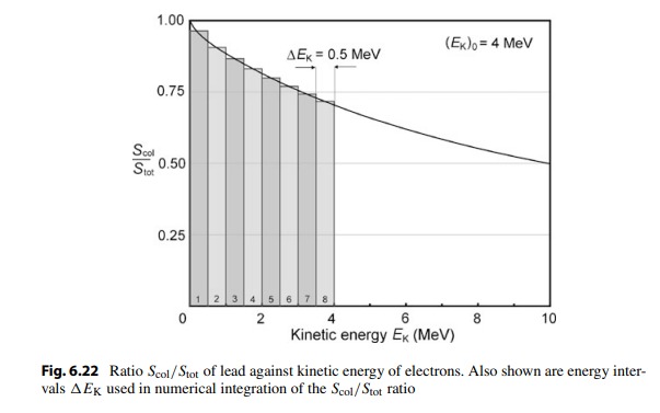
Figure 6.22 shows a plot of the ratio S_{col}/S_{tot} from Table 6.15 against kinetic energy E_K of the electron and it also shows the integration intervals that we used in the numerical integration of S_{col}/S_{tot}, assuming an incident kinetic energy \left(E_K\right)_0 of the electron of 4 MeV. Table 6.17 displays the results of our numerical integration of S_{col}/S_{tot} similar to Table 6.16 that was used in (a) to deal with the numerical integration of S_{col}/S_{tot}. Based on column (6) of Table 6.17 we determine E_{col} for \left(E_K\right)_0 = 4 MeV as follows

E_{\mathrm{col}}=\int_0^{\left(E_{\mathrm{K}}\right)_0} \frac{S_{\mathrm{col}}\left(E_{\mathrm{K}}\right)}{S_{\mathrm{tot}}\left(E_{\mathrm{K}}\right)} \mathrm{d} E_{\mathrm{K}}=\sum_{i=1}^{n=8} \overline{\left(\frac{S_{\mathrm{col}}\left(E_{\mathrm{K}}\right)}{S_{\mathrm{tot}}\left(E_{\mathrm{K}}\right)}\right)_i} \Delta E_{\mathrm{K}}=3.3  \mathrm{MeV}        (6.108)

in excellent agreement with the estimation above that stated E_{\mathrm{col}}=\left(E_{\mathrm{K}}\right)_0-E_{\mathrm{rad}}.

(d) With (6.106) we determined the radiation yield Y\left[\left(E_K\right)_0\right] for initial kinetic energy \left(E_K\right)_0 of 4 MeV. We now use the same relationship (6.106) to plot the radiation yield Y\left[\left(E_K\right)_0\right] against initial kinetic energy \left(E_K\right)_0 in the range 0 ≤ Y\left[\left(E_K\right)_0\right] ≤ 4 MeV and present the appropriate data in column (7) of Table 6.16 as well as in Fig. 6.23. The solid line in the figure represents the NIST data, the data points are determined with (6.106) for a given \left(E_K\right)_0. Our calculated points agree well with the NIST data that show that Y\left[\left(E_K\right)_0\right] increases with initial kinetic energy \left(E_K\right)_0 and asymptotically approaches 100 % at initial kinetic energies above 1000 MeV.