Question 3.AE.13: Voltage ripples due to PWM voltage-source inverters cause vo......
Voltage ripples due to PWM voltage-source inverters cause voltage stress in windings of machines and transformers. The configuration of Fig. E3.13.1 represents a simple winding with two turns consisting of eight segments. Each segment can be represented by an inductance L_i , a resistance R_i , and a capacitance to ground (frame) C_i , and there are four interturn capacitances C_{ij} and inductances L_{ij}. Figure E3.13.2 represents a detailed equivalent circuit for the configuration of Fig. E3.13.1.
a) To simplify the analysis neglect the capacitances C_{ij} and the inductances L_{ij}. This leads to the circuit of Fig. E3.13.3, where the winding is fed by a PWM voltage source (see Fig. E3.13.4). One obtains the 16 differential equations (Eqs. E3.13-1a,b to E3.13-8a, b) as listed below.
\begin{gathered} \frac{d i_1}{d t}=-\frac{R_1}{L_1} i_1-\frac{v_1}{L_1}+\frac{v_s(t)}{L_1},\quad (E3.13-1a) \\ \frac{d v_1}{d t}=\frac{i_1}{C_1}-\frac{G_1}{C_1} v_1-\frac{i_2}{C_1},\quad (E3.13-1b) \\ \frac{d i_2}{d t}=-\frac{R_2}{L_2} i_2-\frac{v_2}{L_2}+\frac{v_1}{L_2},\quad (E3.13-2a) \\ \frac{d v_2}{d t}=\frac{i_2}{C_2}-\frac{G_2}{C_2} v_2-\frac{i_3}{C_2},\quad (E3.13-2b) \\ \frac{d i_3}{d t}=-\frac{R_3}{L_3} i_3-\frac{v_3}{L_3}+\frac{v_2}{L_3},\quad (E3.13-3a) \\ \frac{d v_3}{d t}=\frac{i_3}{C_3}-\frac{G_3}{C_3} v_3-\frac{i_4}{C_3},\quad (E3.13-3b) \end{gathered}.
\begin{aligned} \frac{d i_4}{d t} & =-\frac{R_4}{L_4} i_4-\frac{v_4}{L_4}+\frac{v_3}{L_4},\quad (E3.13-4a) \\ \frac{d v_4}{d t} & =\frac{i_4}{C_4}-\frac{G_4}{C_4} v_4-\frac{i_5}{C_4},\quad (E3.13-4b) \\ \frac{d i_5}{d t} & =-\frac{R_5}{L_5} i_5-\frac{v_5}{L_5}+\frac{v_4}{L_5},\quad (E3.13-5a) \\ \frac{d v_5}{d t} & =\frac{i_5}{C_5}-\frac{G_5}{C_5} v_5-\frac{i_6}{C_5},\quad (E3.13-5b) \\ \frac{d i_6}{d t} & =-\frac{R_6}{L_6} i_6-\frac{v_6}{L_6}+\frac{v_5}{L_6},\quad (E3.13-6a) \\ \frac{d v_6}{d t} & =\frac{i_6}{C_6}-\frac{G_6}{C_6} v_6-\frac{i_7}{C_6},\quad (E3.13-6b) \\ \frac{d i_7}{d t} & =-\frac{R_7}{L_7} i_7-\frac{v_7}{L_7}+\frac{v_6}{L_7},\quad (E3.13-7a) \\ \frac{d v_7}{d t} & =\frac{i_7}{C_7}-\frac{G_7}{C_7} v_7-\frac{i_8}{C_7},\quad (E3.13-7b) \\ \frac{d i_8}{d t} & =-\frac{R_8}{L_8} i_8-\frac{v_8}{L_8}+\frac{v_7}{L_8},\quad (E3.13-8a) \\ \frac{d v_8}{d t} & =\frac{i_8}{C_8}-v_8\left(\frac{1}{Z_8}+\frac{G_8}{C_8}\right) .\quad (E3.13-8b) \end{aligned}The parameters are
Z is either 1 μΩ (short-circuit) or 1 MΩ (open-circuit). As input, assume the PWM voltage-step function v_s(t) (illustrated in Fig. E3.13.4).
Using Mathematica or MATLAB compute all state variables for the time period from t=t_{calculate}=0 to 2.1 ms. Note that for some reason t_{calculate} must be larger than t_{plot}. Plot the voltages (v_s – v_1), (v_1 – v_5), (v_2 – v_6), (v_3 – v_7),\ and\ (v_4 – v_8).
b) For the detailed equivalent circuit of Fig. E3.13.2 establish all differential equations in a similar manner as has been done in part a. As input, assume a PWM voltage-step function v_s(t) (illustrated in Fig. E3.13.4).
Table E3.13.1 Mathematica program list for Application Example 3.13 (part a) for short- circuit with Z=10^{-6}Ω
| Hval=10.01; |
eq1=I1’[t]==-R1/L1*I1[t]-V1[t]/L1+Vs[t]/L1;
|
| Lval=0; | ic1=I1[0]==0; |
| period=200*10^-6; |
eq2=V1’[t]==I1[t]/C1-G1/C1*V1[t]-I2[t]/C1;
|
| duty=0.5; | ic2=V1[0]==0; |
| Vs[t_]:=If[Mod[t,period]< |
eq3=I2’[t]==-R2/L2*I2[t]-V2[t]/L2+V1[t]/L2;
|
| duty*period,Hval,Lval]; | ic3=I2[0]==0; |
| Plot[Vs[t],{t,0,0.001},PlotRange-> |
eq4=V2’[t]==I2[t]/C2-G2/C2*V2[t]-I3[t]/C2;
|
| All,AxesLabel | ic4=V2[0]==0; |
| ->{“t(s)”,“Vs(t)”}] |
eq5=I3’[t]==-R3/L3*I3[t]-V3[t]/L3+V2[t]/L3;
|
| R1=25*10^-6; | ic5=I3[0]==0; |
Table E3.13.1 Mathematica program list for Application Example 3.13 (part a) for short- circuit with Z¼10- 6O—cont’d
| R=25*10^-6; |
eq6=V3’[t]==I3[t]/C3-G3/C3*V3[t]-I4[t]/C3;
|
| R3=25*10^-6; | ic6=V3[0]==0; |
| R4=25*10^-6; |
eq7=I4’[t]==-R4/L4*I4[t]-V4[t]/L4+V3[t]/L4;
|
| R5=25*10^-6; | ic7=I4[0]==0; |
| R6=25*10^-6; |
eq8=V4’[t]==I4[t]/C4-G4/C4*V4[t]-I5[t]/C4;
|
| R7=25*10^-6; | ic8=V4[0]==0; |
| R8=25*10^-6; |
eq9=I5’[t]==-R5/L5*I5[t]-V5[t]/L5+V4[t]/L5;
|
| L1=1*10^-3; | ic9=I5[0]==0; |
| L3=1*10^-3; |
eq10=V5’[t]==I5[t]/C5-G5/C5*V5[t]-I6[t]/C5;
|
| L5=1*10^-3; | ic10=V5[0]==0; |
| L7=1*10^-3; |
eq11=I6’[t]==-R6/L6*I6[t]-V6[t]/L6+V5[t]/L6;
|
| L2=10*10^-3; | ic11=I6[0]==0; |
| L4=10*10^-3; |
eq12=V6’[t]==I6[t]/C6-G6/C6*V6[t]-I7[t]/C6;
|
| L6=10*10^-3; | ic12=V6[0]==0; |
| L8=10*10^-3; |
eq13=I7’[t]==-R7/L7*I7[t]-V7[t]/L7+V6[t]/L7;
|
| L15=5*10^-6; | ic13=I7[0]==0; |
| L37=5*10^-6; |
eq14=V7’[t]==I7[t]/C7-G7/C7*V7[t]-I8[t]/C7;
|
| L26=10*10^-6; | ic14=V7[0]==0; |
| L48=10*10^-6; |
eq15=I8’[t]==R8/L8*I8[t]/L8+V7[t]/L8;
|
| C1=.7*10^-12; | ic15=I8[0]==0; |
| C3=.7*10^-12; |
eq16=V8’[t]==I8[t]/C8-V8[t]*(1/(Z*C8)
|
| C5=.7*10^-12; | #ERROR! |
| C7=.7*10^-12; | ic16=V8[0]==0; |
| C2=7*10^-12; |
sol1=NDSolve[{eq1,eq2,eq3,eq4,eq5,eq6,eq7,
|
| C4=7*10^-12; |
eq8,eq9,eq10,eq11,eq12,eq13,eq14,eq15,eq16,
|
| C6=7*10^-12; |
ic1,ic2,ic3,ic4,ic5,ic6,ic7,ic8,ic9,ic10,ic11,ic12,
|
| C8=7*10^-12; |
ic13,ic14,ic15,ic16},{I1[t],V1[t],I2[t],V2[t],I3[t],
|
| C15=.35*10^-12; |
V3[t],I4[t],V4[t],I5[t],V5[t],I6[t],V6[t],I7[t],V7[t],
|
| C37=.35*10^-12; |
I8[t],V8[t]},{t,0,0.0022},MaxSteps->100000];
|
| C26=3.5*10^-12; |
Plot[Vs[t]-Evaluate[V1[t]/.sol1],{t,0,0.002},
|
| C48=3.5*10^-12; |
AxesLabel->{“Time”, “(Vs-V1) (V)”}]
|
| G1=1/5000; |
Plot[Evaluate[V1[t]/.sol1]-Evaluate[V5[t]/.sol1],
|
| G3=1/5000; |
{t,0,0.002},AxesLabel->{“t(s)”, “(V1-V5) (V)”}]
|
| G5=1/5000; |
Plot[Evaluate[V2[t]/.sol1]-Evaluate[V6[t]/.sol1],
|
| G7=1/5000; |
{t,0,0.002},AxesLabel->{“t(s)”, “(V2-V6) (V)”}]
|
| G2=1/500; |
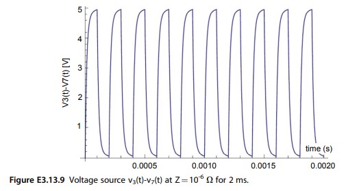
Plot[Evaluate[V3[t]/.sol1]-Evaluate[V7[t]/.sol1],
|
| G4=1/500; |
{t,0,0.002},AxesLabel->{“t(s)”, “(V3-V7) (V)”}]
|
| G6=1/500; |
Plot[Evaluate[V4[t]/.sol1]-Evaluate[V8[t]/.sol1],
|
| G8=1/500; |
{t,0,0.002},AxesLabel->{“t(s)”, “(V4-V8) (V)”}]
|
| Z=1*10^-6; |


Learn more on how do we answer questions.
Solution #1 (Based on Mathematica)
a) Program list for short circuit with Z=10^{-6}Ω is presented in Table E3.13.1 and the cooresponding plots are shown in Figs. E3.13.5 to E3.13.10. Note that the computing time t=t_{calculate}=2.1 ms must be larger than the plot time t=t_{plot}=2 ms.
Program list for open circuit with Z=10^6 Ω is presented in Table E3.13.2 and the cooresponding plots are shown in Figs. E3.13.11 to E3.13.15. Note that the computing time t=t_{calculate}=2.1 ms must be larger than the plot time t=t_{plot} =2 ms.
Table E3.13.2 Mathematica program list for Application Example 3.13 (part a) for open- circuit with Z =10^6 Ω
| Hval=10.; |
eq1=I1’[t]==-R1/L1*I1[t]-V1[t]/L1+Vs[t]/L1;
|
| Lval=0; | ic1=I1[0]==0; |
| period=200*10^-6; |
eq2=V1’[t]==I1[t]/C1-G1/C1*V1[t]-I2[t]/C1;
|
| duty=0.5; | ic2=V1[0]==0; |
| Vs[t_]:=If[Mod[t,period]< |
eq3=I2’[t]==-R2/L2*I2[t]-V2[t]/L2+V1[t]/L2;
|
| duty*period,Hval,Lval]; | ic3=I2[0]==0; |
| Plot[Vs[t],{t,0,0.001},PlotRange-> |
eq4=V2’[t]==I2[t]/C2-G2/C2*V2[t]-I3[t]/C2;
|
| All,AxesLabel | ic4=V2[0]==0; |
| ->{“t(s)”,“Vs(t)”}] |
eq5=I3’[t]==-R3/L3*I3[t]-V3[t]/L3+V2[t]/L3;
|
| R1=25*10^-6; | ic5=I3[0]==0; |
| R2=25*10^-6; |
eq6=V3’[t]==I3[t]/C3-G3/C3*V3[t]-I4[t]/C3;
|
| R3=25*10^-6; | ic6=V3[0]==0; |
| R4=25*10^-6; |
eq7=I4’[t]==-R4/L4*I4[t]-V4[t]/L4+V3[t]/L4;
|
| R5=25*10^-6; | ic7=I4[0]==0; |
| R6=25*10^-6; |
eq8=V4’[t]==I4[t]/C4-G4/C4*V4[t]-I5[t]/C4;
|
| R7=25*10^-6; | ic8=V4[0]==0; |
| R8=25*10^-6; |
eq9=I5’[t]==-R5/L5*I5[t]-V5[t]/L5+V4[t]/L5;
|
| L1=1*10^-3; | ic9=I5[0]==0; |
| L3=1*10^-3; |
eq10=V5’[t]==I5[t]/C5-G5/C5*V5[t]-I6[t]/C5;
|
| L5=1*10^-3; | ic10=V5[0]==0; |
| L7=1*10^-3; |
eq11=I6’[t]==-R6/L6*I6[t]-V6[t]/L6+V5[t]/L6;
|
| L2=10*10^-3; | ic11=I6[0]==0; |
| L4=10*10^-3; |
eq12=V6’[t]==I6[t]/C6-G6/C6*V6[t]-I7[t]/C6;
|
| L6=10*10^-3; | ic12=V6[0]==0; |
| L8=10*10^-3; |
eq13=I7’[t]==-R7/L7*I7[t]-V7[t]/L7+V6[t]/L7;
|
| L15=5*10^-6; | ic13=I7[0]==0; |
| L37=5*10^-6; |
eq14=V7’[t]==I7[t]/C7-G7/C7*V7[t]-I8[t]/C7;
|
| L26=10*10^-6; | ic14=V7[0]==0; |
| L48=10*10^-6; |
eq15=I8’[t]==-R8/L8*I8[t]-V8[t]/L8+V7[t]/L8;
|
| C1=.7*10^-12; | ic15=I8[0]==0; |
| C3=.7*10^-12; |
eq16=V8’[t]==I8[t]/C8-V8[t]*(1/(Z*C8)+G8/C8);
|
| C5=.7*10^-12; | ic16=V8[0]==0; |
| C7=.7*10^-12; |
sol1=NDSolve[{eq1,eq2,eq3,eq4,eq5,eq6,eq7,eq8,
|
| C2=7*10^-12; |
eq9,eq10,eq11,eq12,eq13,eq14,eq15,eq16,ic1,ic2,
|
| C4=7*10^-12; |
ic3,ic4,ic5,ic6,ic7,ic8,ic9,ic10,ic11,ic12,ic13,ic14,
|
| C6=7*10^-12; |
ic15,ic16},{I1[t],V1[t],I2[t],V2[t],I3[t],V3[t],I4[t],
|
| C8=7*10^-12; |
V4[t],I5[t],V5[t],I6[t],V6[t],I7[t],V7[t],I8[t],V8[t]}
|
| C15=.35*10^-12; |
,{t,0,0.0022},MaxSteps->100000];
|
| C37=.35*10^-12; |
Plot[Vs[t]-Evaluate[V1[t]/.sol1],{t,0,0.002},
|
Table E3.13.2 Mathematica program list for Application Example 3.13 (part a) for open- circuit with Z =10^6 Ω—cont’d
| C26=3.5*10^-12; |
AxesLabel->{“Time”, “(Vs-V1) (V)”}]
|
| C48=3.5*10^-12; |
Plot[Evaluate[V1[t]/.sol1]-Evaluate[V5[t]/.sol1],
|
| G1=1/5000; |
{t,0,0.002},AxesLabel->{“t(s)”,“(V1-V5) (V)”}]
|
| G3=1/5000; |
Plot[Evaluate[V2[t]/.sol1]-Evaluate[V6[t]/.sol1],
|
| G5=1/5000; |
{t,0,0.002},AxesLabel->{“t(s)”,”(V2-V6) (V)”}]
|
| G7=1/5000; |
Plot[Evaluate[V3[t]/.sol1]-Evaluate[V7[t]/.sol1],
|
| G2=1/500; |
{t,0,0.002},AxesLabel->{“t(s)”,“(V3-V7) (V)”}]
|
| G4=1/500; |
Plot[Evaluate[V4[t]/.sol1]-Evaluate[V8[t]/.sol1],
|
| G6=1/500; |
{t,0,0.002},AxesLabel->{“t(s)”,“(V4-V8) (V)”}]
|
| G8=1/500; | |
| Z=1*10^6; |