Question 4.AE.3: Engineers are most concerned about the torques generated by ......

a) Balanced Three-Phase Short-Circuit. If the terminals of a synchronous generator are short circuited at rated no-load excitation one obtains the balanced short-circuit currents in per unit [31]:

\begin{aligned} i_a(\varphi)= & \frac{1}{X_d} \cos (\varphi+\alpha)+\frac{\left(X_d-X_d^{\prime}\right)}{X_d X_d^{\prime}} e^{-\varphi / T_d^{\prime}} \cos (\varphi+\alpha) \\ & -\frac{1}{2}\left(\frac{1}{X_d^{\prime}}+\frac{1}{X_q}\right) e^{-\varphi / T a} \cos \alpha-\frac{1}{2}\left(\frac{1}{X_d^{\prime}}+\frac{1}{X_q}\right) e^{-\varphi / T a} . \\ & \cos (2 \varphi+\alpha) \end{aligned}            (E4.3-1)

\begin{aligned} i_b(\varphi)= & \frac{1}{X_d} \cos \left(\varphi+\alpha-120^{\circ}\right)+\frac{\left(X_d-X_d^{\prime}\right)}{X_d X_d^{\prime}} e^{-\varphi / T_d^{\prime}} \\ & \cos \left(\varphi+\alpha-120^{\circ}\right)+\frac{1}{4}\left(\frac{1}{X_d^{\prime}}+\frac{1}{X_q}\right) e^{-\varphi / T a} \cos \alpha \\ & +\frac{1}{2}\left(\frac{1}{X_d^{\prime}}-\frac{1}{X_q}\right) e^{-\varphi / T a} \cos (2 \varphi+\alpha+\delta) \end{aligned}              (E4.3-2)

\begin{aligned} i_c(\varphi)= & \frac{1}{X_d} \cos \left(\varphi+\alpha+120^{\circ}\right)+\frac{\left(X_d-X_d^{\prime}\right)}{X_d X_d^{\prime}} e^{-\varphi / T_d^{\prime}} . \\ & \cos \left(\varphi+\alpha+120^{\circ}\right)+\frac{1}{4}\left(\frac{1}{X_d^{\prime}}+\frac{1}{X_q}\right) e^{-\varphi / T a} . \\ & \cos \alpha+\frac{1}{2}\left(\frac{1}{X_d^{\prime}}-\frac{1}{X_q}\right) e^{-\varphi / T a} \cos (2 \varphi+\alpha-\delta), \end{aligned}            (E4.3-3)

where \tan \delta=\sqrt{3}, \varphi=\omega t.

The field current is

i_f(\varphi)=1+\frac{\left(X_d-X_d^{\prime}\right)}{X_d^{\prime}}\left(e^{-\varphi / T^{\prime} d o}-\cos \varphi e^{-\varphi / T a}\right)            (E4.3-4)

and the torque is

T_{3-\text { phase }}=\frac{\left(X_d^{\prime}-X_q\right)}{2 X_d^{\prime} X_q} \cdot \sin (2 \varphi)+\frac{1}{X_d^{\prime}} \sin \varphi          (E4.3-5)

The maximum torque occurs at the angle φ_{max} which can be obtained from

\cos \varphi_{\max }=\frac{1}{4}\left(\frac{X_q}{X_q-X_d^{\prime}} \pm \sqrt{\left(\frac{X_q}{\left(X_d^{\prime}-X_q\right)}\right)^2+8}\right) .          (E4.3-6)

Figure E4.3.1 illustrates the torque of Eqs. E4.3-5 and E4.3-6.

b) Line-to-Line Short-Circuit. The short-circuit of the two terminals b and c of a synchronous generator results in the line-to-line short-circuit current [31]

or for φ_o=0      i_b=\frac{\sqrt{3}\left(\cos \varphi-\cos \varphi_o\right)}{\left(X_q+X_d^{\prime}\right)-\left(X_q-X_d^{\prime}\right) \cos 2 \varphi}        (E4.3-7)

i_b=\frac{\sqrt{3}(\cos \varphi-1)}{\left(X_q+X_d^{\prime}\right)-\left(X_q-X_d^{\prime}\right) \cos 2 \varphi}              (E4.3-8)

and the torque is

T_{L-L}=-\frac{2}{\sqrt{3}}(\sin \varphi) i_b+\frac{2}{3} \sin 2 \varphi\left(X_d^{\prime}-X_q\right) i_b^2          (E4.3-9)

or

Figure E4.3.2 illustrates the torques of Eqs. E4.3-5, E4.3-6, and E4.3-10.

The open-circuit voltage induced in phase a in case of a short-circuit of line b with line c is

e_a=-\cos \varphi-b\left(\begin{array}{l} \frac{\left[-\sin \varphi \sin 2 \varphi+\left(\cos \varphi-\cos \varphi_o\right) 2 \cos 2 \varphi\right]}{[a-b \cos 2 \varphi]} \\ \frac{\left(\cos \varphi-\cos \varphi_o\right)(\sin 2 \varphi)^2 2 b}{[a-b \cos 2 \varphi]^2} \end{array}\right)                (E4.3-11)

where

a=\left(X_q+X_d^{\prime}\right) \text { and } b=\left(X_q-X_d^{\prime}\right) \text {. }          (E4.3-12a,b)

The maximum value of ea occurs for φ_o=0

Figure E4.3.3 illustrates the induced voltage e_a of Eqs. E4.3-11 and E4.3-12a,b.

c) Line-to-Neutral Short-Circuit. The current when phase a of a synchronous machine at no load is short-circuited is for θ=90°+φ [31]

i_a=\frac{3\left(\cos \theta-\cos \theta_o\right)}{\left(X_q-X_d^{\prime}\right)} \cdot \frac{1}{\frac{\left(X_d^{\prime}+X_q+X_o\right)}{\left(X_q-X_d^{\prime}\right)}-\cos 2 \theta}                    (E4.3-13)

or in terms of an infinite series

\begin{aligned} i_a= & \frac{3\left(\cos \theta-\cos \theta_o\right)}{\left(X_q-X_d^{\prime}\right)} \\ & \frac{2 a}{1-a^2}\left(1+2 a \cos 2 \theta+2 a^2 \cos 4 \theta+\ldots\right), \end{aligned}            (E4.3-14)

where

a=\frac{\sqrt{X_q+\frac{X_o}{2}}-\sqrt{X_d^{\prime}+\frac{X_o}{2}}}{\sqrt{X_q+\frac{X_o}{2}}+\sqrt{X_d^{\prime}+\frac{X_o}{2}}} .              (E4.3-15)

Note that i_a must be initially zero, that is, \varphi=\varphi_o=0 \text { or } \theta_o=90^{\circ}.
The fundamental component becomes now

i_{a 1}=\frac{3 \cos \theta}{X_d^{\prime}+\sqrt{X_q+\frac{X_o}{2}} \cdot \sqrt{X_d^{\prime}+\frac{X_o}{2}}+\frac{X_o}{2}}            (E4.3-16)

or in terms of symmetrical components

i_{a 1}=\frac{3 \cos \theta}{X_d^{\prime}+X_2+X_o}                  (E4.3-17)

d) Out-of-Phase Synchronization. When synchronizing a generator (either machine or inverter) with the power system the following conditions must be met:

• phase sequence must be the same,
• the phase angle between the two voltage systems must be sufficiently small, and
• the slip must be small.

Synchronizing out of phase is an important issue because it generates the highest torques and forces (in particular within the end winding of a machine) when paralleled with the power system [31]. The torque during out-of-phase synchronization is as a function of time φ=ωt and the angle δ between the power system’s voltage and that of the synchronous machine voltage at the time of paralleling:

\begin{aligned} T_{\text {out }-\text { of }-\text { phase }}= & \frac{1}{X_q}[\sin \delta(1-\cos \varphi)+(1-\cos \delta) \sin \varphi] \\ & \left.\left\{1+\frac{\left(X_q-X_d^{\prime}\right)}{X_d^{\prime}}[(1-\cos \delta)(1-\cos \varphi)-\sin \delta \sin \varphi)\right]\right\} . \end{aligned}              (E4.3-18)

Notethis expressionis symmetricalinδ andφ,thatis, δ andφcan beinterchangedwithout altering the relation. Introducing δ=φ in Eq. E4.3-18, one obtains for the torque

\begin{aligned} T_{\text {out-of-phase }}= & \frac{2 \sin \delta(1-\cos \delta)}{X_d^{\prime}}-\sin \delta\left[\frac{X_q-X_d^{\prime}}{X_q X_d^{\prime}}\right] \\ & {\left[2+2 \cos \delta-8(\cos \delta)^2+4(\cos \delta)^3\right] } \end{aligned}              (E4.3-19)

The corresponding field current is

Figure E4.3.4 illustrates the very large torque if the generator is out-of-phase synchronized with the worst case angle of δ=141.5° and when φ=δ in Eq. E4.3-18.
Experimental results [32–34] during out-of-phase synchronization show that for small synchronous machines below 100 kVA a voltage difference of \Delta V \leq \pm 10 \%, a phase angle difference of \Delta \delta \leq \pm 5^{\circ}, \text { and a slip of } s \leq 1 \% can be permitted. For large machines these conditions must be more stringent; that is, the voltage difference \Delta \mathrm{V} \leq \pm 1 \% \text {, the phase angle difference } \Delta \delta \leq \pm 0.5^{\circ} \text {, and the slip } s \leq 0.1 \% \text {. }. During the past first analog [32–34] and then digital paralleling devices have been employed to connect synchronous generators to the grid. Although these devices are very reliable, once in a while a faulty paralleling occurs.
Figure E4.3.5 depicts the various parameters when out-of-phase synchronization occurs with an angle of δ=255° – which is not the worst-case condition (see Fig. E4.3.4). In this analysis subtransient reactances are taken into account.
• Stator currentsia, i_b,\ and\ i_{c} are amplitudemodulated and reach maximum values of 4 pu;
• Zero-sequence component current (i_o=i_a+i_b+i_c) flowing in the grounded neutral is relatively small and about 0.5 pu;
• Electrical generator (G) torque T_G assumes a maximum value of about 4 pu;
• Rotor (torque) angle exceeds 90°;
• Real P_G and reactive Q_G power oscillations occur;
• Slip s reaches values of more than 3 pu; and
• Mechanical torque T_M between generator and turbine is below 1 pu.

Not shown in this graph are the extremely large winding forces in the end region of the stator winding, and the excessive heating of the amortisseur bars and the solid-rotor pole face. The latter issue will be addressed in a later example. In Fig. E4.3.5 the left scale pertains to the dotted signals and the right scale belongs to the full-line signals.
Figure E4.3.6aillustrates the conditions under which a 30 kVA inverter of a wind-power plant was paralleled with the power system [29,30]. The switching frequency and thereforethe fundamental (nominally 60 Hz) frequency was phase-locked withthe power system’s frequency and thus the slip is by definition s¼0. However, the voltage differences and the phase differences must be within certain limits. Experiments showed it was advisable to choose the inverter rms value of the line-to-line voltage always somewhat larger (e.g.,V_{L-Linverter}=260V_{rms})than that of the power system’s line-to-line voltage (e.g.,V_{L-Lpower system}=240 V_{rms}). Figure E4.3.6b depicts the transient current flowing from inverter to power system when inverter is paralleled at an inverter voltage of V_{L-Linverter}=260V_{rms} at an out-of-phase voltage angel of δ=24°, wherethe inverter voltage leads that of the power system. As can be seen, the transient current is more than 200 A. Figure E4.3.7 illustrates the stator flux distribution when a large synchronous generator is paralleled out-of-phase [21]: the stator flux leaves the iron core (stator back iron) and currents are induced in the key bars of the iron-core suspension as well as in the aluminum bars within the dovetails of the iron core. The flux density within the space between the iron core and the frame is 17 mT at a terminal voltage of 1.23 pu. This flux density is sufficient to heat up the solid iron key bars and melt the aluminum bars within the dovetails of the iron core.

e) Synchronizing and Damping Torques. When a synchronous generator is paralleled with the power system one obtains for the angle perturbation Δsin ωt from the steady-state angle δ_0 the synchronizing T_S and damping T_D torques in addition to the steady-state torque T_0 [31]:

T=T_0+T_S(\Delta \sin \omega t)+T_D(\omega \cdot \Delta \cos \omega t)        (E4.3-21)

where

T_0=\frac{V_{\ell-n} \cdot V_{\ell-n o}}{X_d} \sin \delta_0+V_{\ell-n}^2\left[\frac{X_d-X_q}{2 X_q X_d}\right] \sin 2 \delta_0,              (E4.3-22)

where V_{\ell-n o} is the open-circuit phase (line-to-neutral) voltage at steady-state operation, V_{\ell-n o} is the phase (line-to-neutral) voltage during synchronization and is approximately V_{\ell-n o} \approx V_{\ell-n}(\approx 1.0 \mathrm{pu}).

\begin{aligned} & T_S=\frac{V_{l-n} \cdot V_{l-n 0}}{X_d} \cos \delta_0+V_{l-n}^2\left(\frac{1}{X_q}-\frac{1}{X_d}\right) \cos 2 \delta_0 \\ &+V_{l-n}^2 \frac{\left(X_d-X_d^{\prime}\right)}{X_d X_d^{\prime}} \cdot \frac{\left(\omega T_d^{\prime}\right)^2}{1+\left(\omega T_d^{\prime}\right)^2}\left(\sin \delta_0\right)^2, \end{aligned}                  (E4-3.23)

where V_{\ell-n o} is the open-circuit phase (line-to-neutral) voltage at steady-state operation, V_{\ell-n } is the phase (line-to-neutral) voltage during synchronization and is approximately V_{\ell-n o} \approx V_{\ell-n}(\approx 1.0 \mathrm{pu}).

T_D=V_{l-n}^2\left(\sin \delta_0\right)^2\left[\frac{\left(X_d-X_d^{\prime}\right)}{X_d X_d^{\prime}}\right] \frac{T_d^{\prime}}{1+\left(\omega T_d^{\prime}\right)^2}              (E4-3.24)

where

f) Torques during Reclosing. In order to minimize power quality problems after shortcircuits have occurred, it is common practice to reclose the switches that have been opened due to the short-circuit. Short-circuits can be interrupted within four to six 60 Hz cycles. In the hope that the short-circuit has been cleared, the utilities reclose the previously opened switches after nine to fifteen 60 Hz cycles have elapsed. If the short-circuit still persists, then the fault will be cleared again after additional four to six 60 Hz cycles. At the most three to five reclosing operations are performed. The timing of the reclosing is important: if the timing is unfavorable the mechanical torques of the turbine stages become excessive, but under favorable conditions these mechanical torques can be minimized. Only an accurate dynamic calculation can approximately predetermine the most favorable reclosing times. Transient electromagnetic and shaft torques of synchronous generators can become as high as 5–6 during reclosing [35–39]. The magnitudes of the torques depend on the reclosing time. If the reclosing occurs at a time when the electrical torque due to reclosing adds to the transient shaft torque, the resulting mechanical shaft becomes large as comparedto the case where the electrical torque due to the reclosing opposes the transient shaft torque; in the latter case the resulting shaft torque will be relatively small. This amplification effect of the mechanical transient torque has its analogy in the “swing effect” one encounters on a playground.

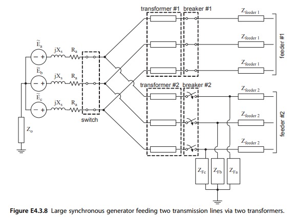
Joyce et al. [35,36] have recommended introducing a measure for the theoretical lifetime of a turbine shaft: the occurrence of many high torsional torques reduces the lifetime of a shaft more quickly than the occurrence of low torsional torques. Figure E4.3.8 illustrates a common connection of a power plant to the high-voltage system. One generator feeds two transformers, which are connected to high-voltage feeders each. This is to minimize the outage of a power plant due to external faults such as short-circuits within the power system. The short-circuit is caused by making the impedances Z_{Fa}, Z_{Fb},\ and\ Z_{Fc} zero. Breaker #2 interrupts the short-circuit and recloses after a preprogrammed time.

Figures E4.3.9a and E4.3.9b depict the various parameters when reclosing with different reclosing times but with the same short-circuit duration (104 ms) occurs. In these graphs the left scale pertains to the dotted signals and the right scale belongs to the full-line signals.

Summarizing one can state the following:

• During the three-phase short-circuit the stator currents i_a,\ i_b,\ and\ i_c are amplitude modulated and exceed maximum values of 4 pu;
• Zero-sequence component current (i_o=i_a+i_b+i_c) flowing in the grounded neutral is relatively large and exceeds 4 pu;
•Electrical torque T_G assumes a maximum value of about 3 pu;
•Rotor (torque) angle is below 90°;
• Very large (about 2 pu) real P_G and reactive Q_G power swings occur;
• Maximum slip reaches values of more than 1 pu;
• Mechanical torque T_M between generator and turbine is below 1 pu, but it has an alternating component causing mechanical stress; and
•In both cases the stability of the synchronous generators is maintained due to the torque angle δ being less than 90°.

Not shown in the graphs are the extremely large winding forces in the end region of the stator winding, and the excessive heating of the amortisseur bars residing on the rotor. As can be expected, the electrical and mechanical stresses depend on the reclosing times, which are 450 ms and 745 ms for Figs. E4.3.9a and E4.3.9b, respectively.