Consider the transfer function model of Exercise 20.1. For each of the four sets of design parameters shown below, design a model predictive controller. Then do the following: (a) Compare the controllers for a unit step change in set point. Consider both the y and u responses. (b) Repeat the

Chapter 20 Q. 20.4

Process Dynamics and Control-Solution Manual [EXP-2817]

Consider the transfer function model of Exercise 20.1. For each of the four sets of design parameters shown below, design a model predictive controller. Then do the following:

(a) Compare the controllers for a unit step change in set point. Consider both the $y$ and $u$ responses.

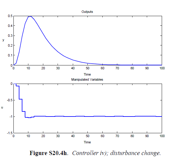
(b) Repeat the comparison of (a) for a unit step change in disturbance, assuming that $G_{d}(s)=G(s)$ .

Set No.	Δt	N	M	P	R
(i)	2	40	1	5	0
(ii)	2	40	20	20	0
(iii)	2	40	3	10	0.01
(iv)	2	40	3	10	0.1

Step-by-Step

Report Solution

Verified Solution

The step response is obtained from the analytical unit step response as in Example 20.1. The feedback matrix $K _{c}$ is obtained using Eq. $20-65$ as in Example 20.5. These results are not reported here for sake of brevity. The closed-loop response for set-point and disturbance changes are shown below for each case. The MATLAB MPC Toolbox was used for the simulations.

$K _{c} \triangleq\left( S ^{T} Q S + R \right)^{-1} S ^{T} Q$ (20-65)

i) For this model horizon, the step response is over $99 \%$ complete as in Example 20.5; hence the model is good. The set-point and disturbance responses shown below are non-oscillatory and have long settling times

ii) The set-point response shown below exhibits same overshoot, smaller settling time and undesirable “ringing” in $u$ compared to part i). The disturbance response shows a smaller peak value, a lack of oscillations, and faster settling of the manipulated input.

iii) The set-point and disturbance responses shown below show the same trends as in part i).

iv) The set-point and load responses shown below exhibit the same trends as in parts (i) and (ii). In comparison to part (iii), this controller has a larger penalty on the manipulated input and, as a result, leads to smaller and less oscillatory input effort at the expense of larger overshoot and settling time for the controlled variable.