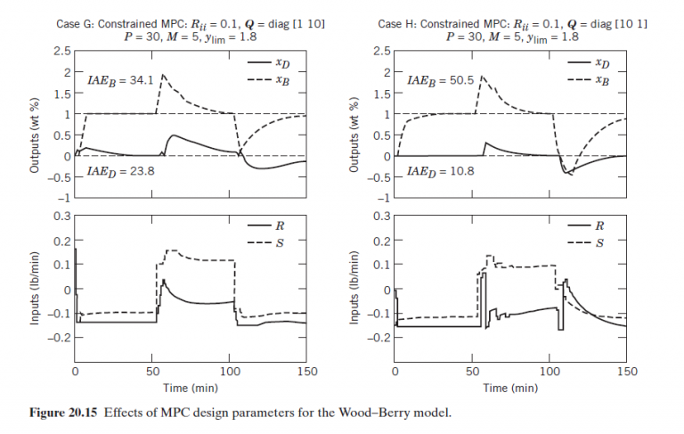
In Section 20.6.1, MPC was applied to the Wood-Berry distillation column model. A MATLAB program for this example and constrained MPC is shown in Table E20.8. The design parameters have the base case values (Case B in Fig. 20.14) except for P=10 and M=5. The input constraints are the saturation limits for each input (-0.15 and +0.15 ). Evaluate the effects of control horizon M and input weighting matrix R by simulating the set-point change and the first disturbance of Section 20.6.1 for the following parameter values:
(a) Control horizon, M=2 and M=5
(b) Input weighting matrix, R =0.1 I and R = I Consider plots of both inputs and outputs. Which choices of M and R provide the best control? Do any of these MPC controllers provide significantly better control than the controllers shown in Figs. 20.14 and 20.15? Justify your answer.
| Table E20.8 MATLAB Program (Based on a program by Morari and Ricker (1994)) |
| g11=poly2tfd(12.8,[16.7 1],0.1); % model |
| g21=poly2tfd(6.6,[10.9 1],0,7); |
| g12=poly2tfd(−18.9,[21.0 1],0,3); |
| g22=poly2tfd(−19.4,[14.4 1],0,3); |
| gd1=poly2tfd(3.8,[14.9 1],0,8.1); |
| gd2=poly2tfd(4.9,[13.2 1],0,3.4); |
| tfinal=120; % Model horizon, N |
| delt=1; %Sampling perio |
| ny=2; %Number of outputs |
| model=tfd2step(tfinal,delt,ny,g11,g21,g12,g22) |
| plant=model; %No plant/model mismatch |
| dmodel=[ ] %Default disturbance model |
| dplant=tfd2step(tfinal,delt,ny,gd1,gd2) |
| P=10; M=5; % Horizons |
| ywt=[1 1]; uwt=[0.1 0.1];%Q and R |
| tend=120; % Final time for simulation |
| r=[0 1]; %Set-point change in XB |
| a=zeros([1,tend]); |
| for i=51:tend |
| a(i)=0.3∗2.45; %30 %step in F at t=50 min. |
| end |
| dstep=[a′]; |
| ulim=[−.15 −.15 .15 .15 1000 1000];%u limits |
| ylim=[ ]; %No y limits |
| tfilter=[ ]; |
| [y1,u1]=cmpc(plant,model,ywt,uwt,M,P,tend,r, |
| ulim,ylim, tfilter,dplant,dmodel,dstep); |
| figure(1) |
| subplot(211) |
| plot(y1) |
| legend(′XD′,′XB′) |
| xlabel(′Time (min)′) |
| subplot(212) |
| stairs(u1)% Plot inputs as staircase functions |
| legend(′R′,′S′) |
| xlabel(′Time (min)′) |