Question 3.17: Lubricated Shaft Rotation with Heat Generation Consider “cyl......
Lubricated Shaft Rotation with Heat Generation
Consider “cylindrical” Couette flow where, somewhat similar to Example 3.15, the rotating shaft \rm(R_i , ω_i ) is adiabatic and the stationary housing \rm(R_0, T_0 ) is isothermal. In light of viscous dissipation, find T(r) as well as \rm T_{max} at \rm r =R_i and \rm\hat Q_{wall}(r=R_0).
| Approach | Assumptions | Sketch |
| • Reduced Θ- momentum equation | • Steady laminar 1-D axisymmetri cal flow |  |
| • Postulate \rm v_θ=v_θ(r) only | • No gravity or end effects | |
| • Constant properties |
Learn more on how do we answer questions.
Based on the postulate and assumptions, the Continuity Equation is satisfied and the Θ-momentum equation in cylindrical coordinates reduces to (see Equation Sheet in App. A):
{\frac{\mathrm{d}}{\mathrm{d}\mathrm{r}}}\left\lgroup{\frac{1}{\mathrm{r}}}{\frac{\mathrm{d}}{\mathrm{d}\mathrm{r}}}\left(\mathrm{r}\,\mathrm{v}_{\theta}\right)\right\rgroup =0 (E.3.17.1a)
subject to
\rm v_\theta (r=R_i)=(\omega R)_i~~\text{and}~~v_\theta (r=R_0)=0 (E.3.7.1b,c)
Double integration and invoking the B.C.s yields:
\rm \mathrm{v_{\theta }(r)=\frac{\omega_{i}^{}\,{R_{i}}_{}({ R_{0}}^{{}}/{R_{i}}_{}{{}})^{2}}{\left\lgroup\frac{{ R_{0}}}{{ R_{i}}}\right\rgroup^{2}-1}\left[\frac{ R_{i}}{\mathrm{r}}-\frac{\mathrm{r}}{\mathrm{R}_{\mathrm{i}}{}}\right]} (E.3.17.2)
The heat transfer equation (see Equation Sheet in App. A) reduces to:
0=\frac{\mathrm{k}}{\mathrm{r}}\,\frac{\mathrm{d}}{\mathrm{d}\mathrm{r}}\!\left\lgroup\mathrm{r}\,\frac{\mathrm{d}\mathrm{T}}{\mathrm{d}\mathrm{r}}\right\rgroup\!-\!\mu\Phi (E.3.17.3a)
where
\rm\Phi=\left\lgroup{\frac{\mathrm{d}\mathrm{v_{\theta}}}{\mathrm{d}\mathrm{r}}}-{\frac{\mathrm{v_{\theta}}}{\mathrm{r}}}\right\rgroup^{2} (E.3.17.3b)
and as stated:
\rm\left.{\frac{\mathrm{d}T\ }{\mathrm{d}\mathrm{r}}}\right|_{\mathrm{r}=\mathrm{R_i}}=0;~\mathrm{T}(\mathrm{r}=\mathrm{R}_{0})=\mathrm{T}_{0}{} (E.3.17.3c,d)
With \rm v_\theta (r) given, Eq. (E.3.17.3b) can be determined and hence Eq. (E.3.17.3a) can be integrated subject to Eq. (E.3.17.3c, d). Thus,
Now, either by inspection of (E.3.17.4) or setting dT/dr to zero, \rm T_{max} occurs at \rm r = R_i. In dimensionless form,
\rm\frac{T_{\mathrm{max}}-T_{0}}{\frac{\mu}{4k}\left[\frac{2\omega _iR_i}{1-\left\lgroup\frac{R_i}{R_0} \right\rgroup^2 } \right]^2 }=\Bigg[\left\lgroup \frac{\mathrm{R}_{\mathrm{i}}}{\mathrm{R}_{0}}\right\rgroup ^{2}-1+2\mathrm{ln}\left\lgroup \frac{\mathrm{R}_{\mathrm{o}}}{\mathrm{R}_{\mathrm{i}}}\right\rgroup \Bigg] (E.3.17.5)
The wall heat transfer rate per unit length is:
\rm \hat{{ Q}}_{\mathrm{~wall}}=(2\pi{ R_{0}})~\mathrm{q}({r}={ R_{0}});where \rm\mathrm{{q}}(\mathrm{r}=\mathrm{R}_{0})=-\mathrm{k}\left.{\frac{\mathrm{{d}}T}{\mathrm{{d}}\mathrm{r}}}\right|_{\mathrm{{r=R_0}}}\, (E.3.17.6a, b)
Hence,
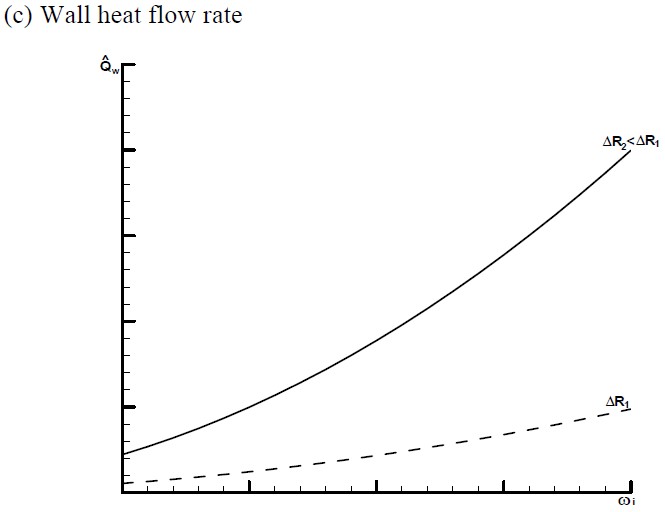
\rm \hat{\mathrm{Q}}_{\mathrm{w}}=\frac{4\pi\mathrm{\mu}(\mathrm{\omega }\mathrm{R})_{\mathrm{i}}^{2}}{1-\left\lgroup\frac{\mathrm{R}_{\mathrm{i}}}{\mathrm{R}_{0}}\right\rgroup^{2}} (E.3.17.6c)
Graphs:
Comments:
• For small gaps, i.e., \rm R_o − R_i << 1, the velocity profiles are almost linear, despite the hyperbolic term in Eq. (E.3.17.2). Clearly, with ΔR << 1, \rm v_θ (r) is “linearized”.
• This is not the case for T(r) due to the strong viscous (heating effect (see Graph b).
• As expected, \rm\hat Q_w(\omega _i) decreases with a strong nonlinear influence of the gap size (see Graph c)